In a previous post, I discussed spatial econometric modeling and how spatial regression models can be used to account for various types of spatial dependence in the data. In many data analyses, we often face the issue of not knowing the true model from which our data is generated. To resolve this model uncertainty issue, general practice is to perform model selection. This is done by fitting a set of candidate models and comparing their fit statistics using some criteria such as Akaike information criterion (AIC) and Schwarz information criterion (SBC). Among those candidate models, the model with the best fit statistic is chosen to be the winner.

For spatial regression analysis, the CSPATIALREG procedure in SAS^® Econometrics automates the model selection process for SAS users. First, I will introduce how to construct spatial weights matrices based on contiguity and distance measures. Then I will demonstrate how PROC CSPATIALREG can be used to automate spatial regression model selection.

Boston housing data

To demonstrate the spatial regression model selection feature in PROC CSPATIALREG, consider the Boston housing data. It was initially presented by Harrison and Rubinfeld (1979) and then later corrected and augmented by Gilley and Pace (1996). The data contains the housing information for 506 census tracts in Boston from the 1970 census. For illustration purposes only, we consider four variables in the data as follows:

• MedValue: median value (measured in $1,000) of owner-occupied homes per census tract on a log scale
• PTRatio: pupil-teacher ratio per town on a log scale
• Status: percentage of the population with lower status on a log scale
• Tract: census tract ID

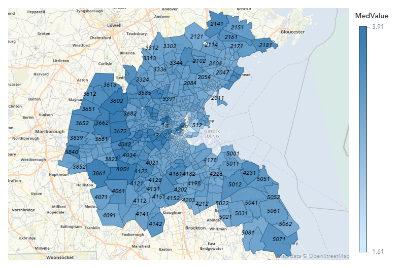
The response variable MedValue and two independent variables, PTRatio and Status, are used in the subsequent spatial econometric models. Using SAS^® Visual Analytics, Figure 1 displays log-transformed median housing values (i.e., MedValue) for 506 census tracts in Boston. As shown in Figure 1, housing values for neighboring census tracts tend to be similar. This is an indication of spatial dependence in the data. This spatial dependence motivates you to consider spatial econometric models for analyzing the data. Before we proceed with spatial econometric models, we need to create a spatial weights matrix to describe the neighbor relationship between two census tracts.

Creating spatial weights matrix

Spatial weights matrices play an important role in spatial econometric modeling because they describe neighbor relationships between different observation units. More importantly, spatial weights matrices are used to formulate various types of spatial dependence in spatial econometric models. To create a spatial weights matrix, you can use neighbor criteria such as contiguity measure, distance measure, etc.

For the contiguity criterion, two observation units are neighbors to each other if they share a common border. For the Boston housing data, you can use the autocall macro in SAS^® STAT to compute the adjacent census tracts and the number of neighbors for each census tract as follows:

%NEIGHBOR("boston_tracts.shp", IDVAR=tract, OUTNBRS=neighbor, OUTADJ=adjacent)

The first argument to the %NEIGHBOR macro is the path to the shapefile for census tracts in Boston (named boston_tracts.shp). You use the IDVAR= option to specify an ID variable that identifies each census tract. The OUTNBRS= and OUTADJ= options enable you to specify the name of a SAS data set to store adjacent census tracts and the number of neighbors for each census tract, respectively.  The output SAS data set adjacent, containing adjacent census tracts from %NEIGHBOR macro, the following %CONTIGUITY macro creates a sparse representation of the spatial weights matrix based on the contiguity criterion. The resulting spatial weights matrix is called W1.

%CONTIGUITY(adjacent, OUTWS=W1)

You can also use a distance measure to define neighbor relationships between two observation units. As an example, the %DISTANCE macro takes the shapefile for census tracts in Boston and the ID variable that identifies each census tract as inputs. It then creates a sparse spatial weights matrix using the K-nearest neighbor criterion with K=6.

%DISTANCE("boston_tracts.shp", IDVAR=tract, K=6, OUTWS=W2)

In the %DISTANCE macro, you compute the pairwise geodetic distance between a census tract and the remaining census tracts based on their longitude and latitude coordinates. These pairwise distances are then sorted in ascending order. Only census tracts that are K-nearest neighbors to the census tract are considered its neighbors. The resulting spatial weights matrix W2 has three columns. The first two columns refer to census tract IDs for neighbor pairs. The last column is all ones to indicate a neighbor relationship.

Automatic model selection

After creating a spatial weights matrix, you can use it for fitting multiple models and identify which model best describes the data. In PROC CSPATIALREG, you can use the TYPE=AUTO or TYPE=ALL options in the MODEL statement to fit multiple models and to perform model selection.

The following SAS statements fit seven models, SAC, SARMA, SAR, SEM, SMA, CAR, and LINEAR, using the contiguity-based spatial weights matrix W1. The IMPACT option is specified to request the impact estimates table. This enables you to infer the marginal effects of each explanatory variable in a model.

   data sascasl.Boston;
      set Boston;
   run;
________________________________________________________
   data sascasl.W1;
      set W1;
   run;
________________________________________________________
   proc cspatialreg data=sascasl.Boston wmat=sascasl.W1
      impact (nmc=5000 order=50);
      model MedValue=PTRatio Status/type=auto;
      spatialid Tract;
   run;

Table 1 presents fit statistics such as log-likelihood value, AIC, SBC, and other information for the seven models being fit. The status code of 0 indicates convergence has been reached for optimization, according to the convergence criterion in the Reason column. If AIC or SBC is used for model selection, SAC is the winner because it has the smallest value of AIC or SBC.

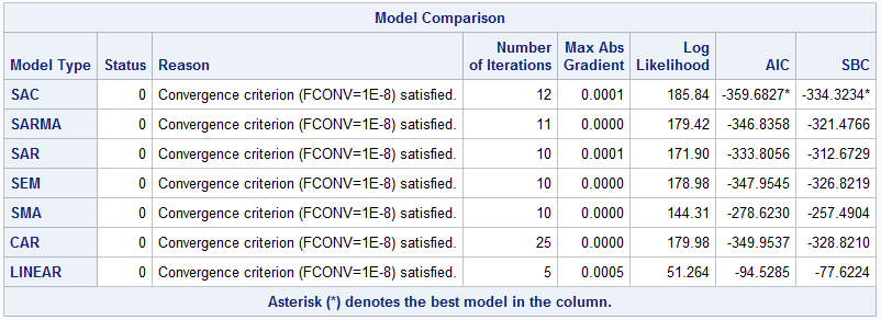
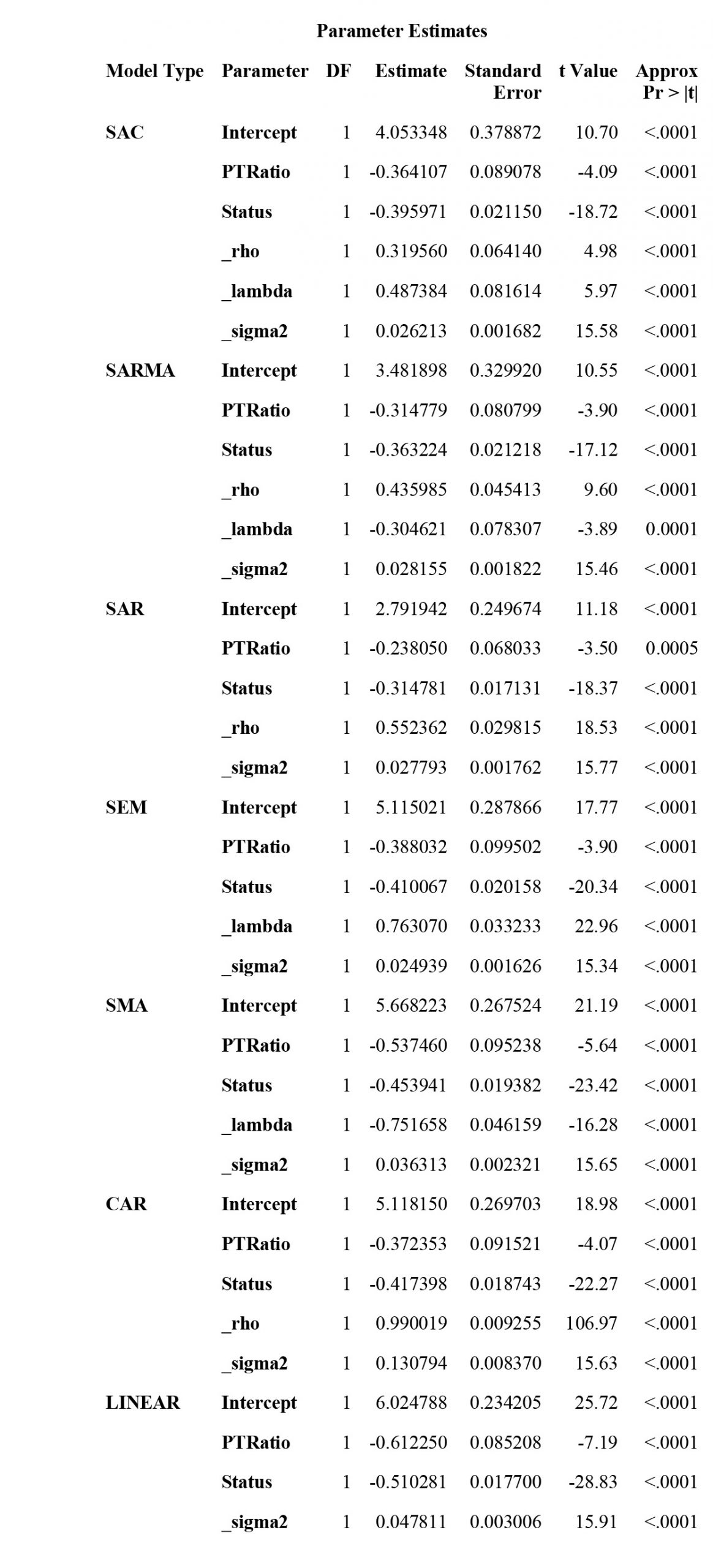
Table 2 presents parameter estimates for the models. According to parameter estimates for SAC model, the spatial coefficient _rho is positive and significant at 0.05 level. So you can conclude that median home values of a census tract are positively impacted by those of its neighboring census tracts. In addition, the regression coefficients for PTRatio and Status are both negative and significant at 0.05 level. This suggests a negative relationship between each of these two covariates and the response variable.

Regression coefficients in spatial econometric models don’t have the same interpretation as their counterparts in classical linear regression models. To correctly interpret marginal effects in spatial econometric models, you need to examine the summary of average direct, average indirect, and average total effects.  Table 3 presents the average direct, average indirect, and average total effects for PTRatio and Status in each of the models.

For the winning model (i.e., SAC model), you conclude that both PTRatio and Status have significant and negative direct, indirect, and total effects. Given that the dependent variable and two explanatory variables are on a log scale, you can conclude that a 1% increase in pupil-teacher ratio leads to a total of 0.537% decrease in median home values. Similarly, a 1% increase in the percentage of the population with lower status leads to a total of 0.586% decrease in median home values.

Because they don’t include spatial lagged explanatory variables in the regression, the preceding models don’t account for local spillover effects. To account for this, you can fit the other seven models in PROC CSPATIALREG (SDAC, SDARMA, SDM, SDEM, SDMA, CAR2, and SLX) by specifying a SPATIALEFFECTS statement, as shown below.

   proc cspatialreg data=sascasl.Boston wmat=sascasl.W1
      impact (nmc=5000 order=50);
      model MedValue=PTRatio Status/type=auto;
      spatialeffects PTRatio Status;
      spatialid Tract;
   run;

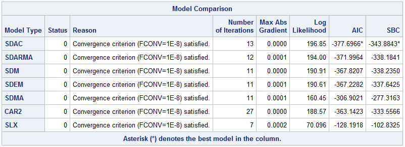
Table 4 presents fit statistics for the SDAC, SDARMA, SDM, SDEM, SDMA, CAR2, and SLX models. If AIC or SBC is used for model selection, SDAC is the winning model among these seven models (in Table 4) since it has the smallest AIC or SBC. Among all 14 models listed in Table 1 and Table 4, the SDAC model has the smallest values of AIC and SBC. As a result, by AIC or SBC criterion, the SDAC model is the winning model that best describes the Boston housing data.

The models in Table 1 and Table 4 represent the complete list of models that are supported in PROC CSPATIALREG. Together, these account for various forms of spatial dependence in the data. However, in many cases, you don’t know the exact forms of spatial dependence in your data before conducting the analysis. In those cases, you can fit all 14 models by using the TYPE=ALL option and a SPATIALEFFECTS statement shown below.

   proc cspatialreg data=sascasl.Boston wmat=sascasl.W1
      impact (nmc=5000 order=50);
      model MedValue=PTRatio Status/type=all;
      spatialeffects PTRatio Status;
      spatialid Tract;
   run;

Conclusion

One key component in spatial econometric modeling is the construction of spatial weights matrices. The other is the choice of a spatial regression model. To explore different structures of spatial dependence in the data, spatial weights matrices are often created based on some commonly accepted neighbor criteria. To ensure correct parameter estimates and inference, it is vital to choose a spatial regression model that best describes underlying spatial dependence in the data.

We have demonstrated how to create spatial weights matrices from a shapefile. We used two commonly used neighbor criteria: the contiguity and distance measures. Automatic model selection in PROC CSPATIALREG enables SAS users to fit and compare multiple models. It also enables the identification of a model that best describes their data according to some model selection criteria. SAS provides the CSPATIALREG procedure and macros with our products. These enable our users to perform their spatial econometric modeling in a cohesive, efficient, and best practices manner.

References

Harrison, D., and Rubinfeld, D. (1978) Hedonic prices and the demand for clean air. Journal of Environmental Economics and Management, 5, 81—102.
Gilley, O., and Pace, R. (1996). On the Harrison and Rubinfeld Data, Journal of Environmental Economics and Management, 31, 403—405.