Note from Udo Sglavo: In our peace of mind blog series, we documented areas of analytics that are either evolving or not necessarily in the standard toolset of data scientists. We looked at causal modeling, network analytics, and econometrics, to name a few. With this blog post, we would like to draw your attention to spatial econometric modeling. Wouldn't it be great to go beyond simple map visualizations by integrating location data into your analytical tasks? Senior research statistician developer Guohui Wu shares new perspectives in understanding how events occurring in one location are affected by events occurring in neighboring locations.

Decision making and spatial analysis

Due to the increasing popularity of spatial data, the demand for spatial analysis has surged in the past few decades. Geographical information in spatial data provide you with new perspectives in understanding how events occurring in one location are affected by events occurring in neighboring locations.

In this post, I will present an overview on spatial econometric analysis. I will also introduce the SPATIALREG procedure in SAS/ETS^® and the CSPATIALREG procedure in SAS^® Econometrics in SAS® Viya®. Both of these can be used for analyzing a wide range of spatial econometric models.

Spatial data and spatial econometrics

Typically, spatial data refers to any data that contains information about specific locations in space.  As observations in time series are referenced by time, observations in spatial data are geographically referenced.  For example, geographic information such as longitude-latitude coordinates, zip codes, street address, and census tract codes allows us to identify different points or regions on earth.

From an analytic point of view, spatial data invalidate the underlying assumption of independence between observations for standard linear regression models. This is because data collected over different locations or regions in space are often spatially correlated. The strength of spatial correlation is determined by the proximity of two spatial units in space. The two observations are more correlated when two spatial units are closer.

Ignoring spatial dependence in the data can lead to biased parameter estimates and flawed inference. Spatial data analysis aims to account for spatial dependence in the data. This ensures the resulting parameter estimates and inference are correct. Combining spatial analysis and econometrics, spatial econometrics extends standard regression models by explicitly incorporating spatial effects for cross-sectional and panel data. These extended regression models deal with two specifications of spatial effects - spatial interaction and spatial heterogeneity. They are often referred to as spatial econometric models.

What is spatial econometric analysis?

As illustrated by the flowchart below, spatial econometric analysis often involves three steps. You begin spatial econometric analysis with data preparation and exploratory data analysis prior to the model fitting. In the second step of model fitting, the actions in sequence are:

1. choosing a model to fit to the data
2. estimating the model
3. performing model diagnostic checks

The third step relates to post-model-fitting inference such as computing fitted values and marginal effects.

Spatial data mapping and processing

To prepare data for your analysis, some dedicated tools are required to import, project, aggregate, and visualize spatial data. Depending on what operations that you need when processing your data, various SAS mapping procedures can be used to meet your needs.

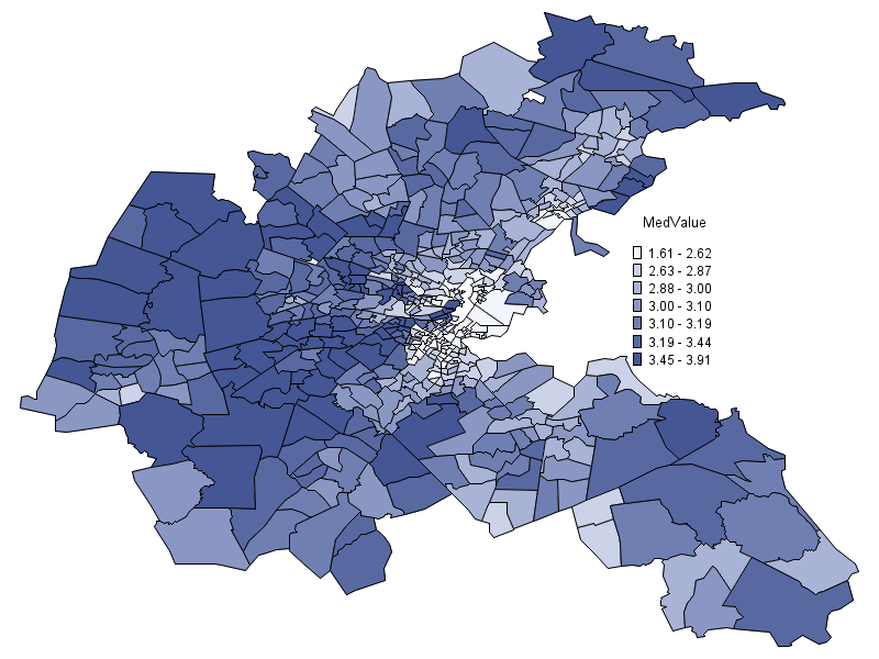
Although spatial data come in various formats, the shapefile format is widely used to store geometry and attribute information of spatial features such as points, lines, and polygons. You can use the MAPIMPORT procedure to read shapefiles in SAS. To visualize your data, you can use both GMAP and SGMAP procedures to show variations of a variable between geographic areas on a map. For example, Figure 2 displays median log-transformed home values for 506 census tracts in Boston from 1970 census (Harrison 1978) using PROC GMAP.

If your data contains address information, the GEOCODE procedure can be used to convert an address to geographic coordinates (longitude and latitude). Based on geographic coordinates, you can compute the distance between two locations and project the longitude-latitude coordinates to a 2-dimensional plane with several map projection techniques provided in the GPROJECT procedure. You use the GREMOVE and GREDUCE procedure to combine unit areas and reduce the number of points in a map data set, respectively. SAS^® Visual Analytics also provides Location Analytics capabilities to leverage geographic potential of your data. This includes data visualization, geocoding, geographic selection, geo-searching, and much more.

After some data cleansing and exploratory data analysis, you are ready to fit some spatial econometric models to your data. The two key components are constructing spatial weights matrices and choosing a model.

The spatial weights matrix W

Spatial weights matrices play an important role in spatial econometric modeling. They are used to describe the proximity of spatial units and to formulate spatial econometric models. In its simplest form, a spatial weights matrix W is an $n \times n$ binary matrix with the $(i,j)$th entry $W_{ij}$ being

$$W_{ij} = \begin{cases} 1, &\text{if units $i$ and $j$ are neighbors} \\0, &\text{if units $i$ and $j$ are not neighbors} \end{cases}$$

where $n$ is the number of spatial units in the data. By convention, $W_{ii}=0$ because you normally do not consider a spatial unit $i$ a neighbor of itself.
To define neighbor relationships between spatial units, some neighbor criteria need to be chosen. In practice, you can consider neighbor criteria to be based on contiguity, distance, and many other factors.

Spatial econometric modeling

For continuous data, the standard linear regression model is useful for modeling the linear relationship between a response variable and some explanatory variables. For instance, in a vector form, the linear regression model can be described as

$\mathbf{ y=X_1}\boldsymbol{ \beta+\epsilon.}$

Spatial econometric models extend the standard linear regression model by incorporating spatial dependence arising from three different interaction effects:

• Endogenous interaction effect: $y_i$ depends on $y_j$ in a neighboring region
• Exogenous interaction effects: $y_i$ depends on $x_j$ in a neighboring region
• Interaction effect among error terms: $\epsilon_i$ depends on $\epsilon_j$ of a neighboring region

The linear regression model can be extended by including the spatially lagged dependent variable Wy as an additional regressor to account for endogenous interaction effect. This leads to a spatial autoregressive (SAR) model of the form:

$\mathbf{ y=}\mathrm{ \rho}\mathbf{ Wy+X_1}\boldsymbol{ \beta+\epsilon.}$

Similarly, spatially lagged explanatory variables in the form of WX are included in the linear regression model to address exogenous interaction effects. In this case, you end up with the following model:

$\mathbf{ y=X_1}\boldsymbol{\beta+}\mathbf{WX_2}\boldsymbol{ \gamma+\epsilon.}$

For spatial dependence in the error terms, the linear regression model can be extended by assuming the error terms follow specific structures, such as the spatial autoregressive and spatial moving average structure.

Due to presence of interaction effects, regression coefficients $\boldsymbol{ \beta}$ in spatial econometric models do not necessarily have the same interpretation as in the standard linear regression model. As a result, marginal effects are often computed to quantify how much change you would expect for changes in explanatory variables. To this end, three impact estimators are provided to summarize the direct impact, indirect impact, and total impact of changes arising from explanatory variables on the dependent variable.

SPATIALREG procedure and the CSPATIALREG procedure

Both the SPATIALREG procedure and the CSPATIALREG procedure can be used for spatial econometric modeling. The CSPATIALREG procedure is designed to run on a cluster of machines that distribute the data and the computations. The SPATIALREG procedure runs on a single machine. Table 1 provides a complete list of spatial regression models in the CSPATIALREG procedure. The CSPATIALREG procedure is capable of handling large spatial data. In addition, it supports features such as parameter estimation, hypothesis testing, marginal effects computation, and many more. The SPATIALREG procedure supports similar features to the CSPATIALREG procedure except for conditional autoregressive models and impact estimation.

The modeling capabilities in the SPATIALREG and CSPATIALREG procedures give you the analytical power to unleash the geographic potential of your data and gain actionable insights from it.

Here's resources to learn more:

• Big Value from Big Data: SAS/ETS^® Methods for Spatial Econometric Modeling in the Era of Big Data
• Add the “Where” to the “What” with Location Analytics in SAS^® Visual Analytics 8.3
• SAS Mapping Procedures documentation
• The CSPATIALREG Procedure documentation
• Introduction to Spatial Econometric Modeling
• Spatial Econometric Modeling for Big Data Using SAS/Econometrics

This is the tenth post in our series about statistics and analytics bringing peace of mind during the pandemic.