Linear programming (LP) and mixed integer linear programming (MILP) solvers are powerful tools. Many real-world business problems, including facility location, production planning, job scheduling, and vehicle routing, naturally lead to linear optimization models.

Sometimes a model that is not quite linear can be transformed to an equivalent linear model to reduce the overall computational time. Experienced modelers have learned a bag of tricks to accomplish such linearization by introducing new variables and constraints. A recently added feature automates some of these tricks by performing the necessary transformations on your behalf.

The LINEARIZE option in SAS Optimization

Since December 2020, in SAS Optimization in SAS Viya, OPTMODEL has included a LINEARIZE option to automate linearization for several common use cases:

• Product of binary variables.
• Product of binary variables and a bounded variable.
• MIN, MAX, and absolute value.
• Bounds on a ratio of linear functions.

In this blog post, I'll demonstrate the LINEARIZE option in the context of a maximum dispersion problem. For example, where should you build a fixed number of new stores from a set of candidate locations? Or where should you build new distribution centers to improve a regional supply chain?

Maximum dispersion problem

In his Yet Another Mathematical Programming Consultant blog, Erwin Kalvelagen described the maximum dispersion problem as follows:

Given $n$ points with their distances $d_{i,j}$, select $k$ points such that the sum of the distances between the selected points is maximized.

A natural way to model this problem is to introduce a binary decision variable $s_i$ to indicate whether point $i$ is selected and then maximize the quadratic function $\sum_{1 \le i < j \le n} d_{i,j} s_i s_j$ subject to a linear constraint $\sum_{i=1}^n s_i = k$. This nonconvex mixed integer quadratic programming (MIQP) problem is difficult to solve. Kalvelagen shows how it can be linearized and solved quickly with a MILP solver.

Input data

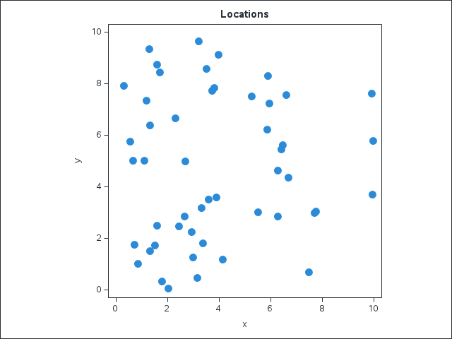
The following DATA step contains the input data for $n=50$ locations, with coordinates $x$ and $y$:

/* store the input data in a data set */
data indata;
   input point $ x y;
   datalines;
i1        1.717       8.433
i2        5.504       3.011
i3        2.922       2.241
i4        3.498       8.563
i5        0.671       5.002
i6        9.981       5.787
i7        9.911       7.623
i8        1.307       6.397
i9        1.595       2.501
i10       6.689       4.354
i11       3.597       3.514
i12       1.315       1.501
i13       5.891       8.309
i14       2.308       6.657
i15       7.759       3.037
i16       1.105       5.024
i17       1.602       8.725
i18       2.651       2.858
i19       5.940       7.227
i20       6.282       4.638
i21       4.133       1.177
i22       3.142       0.466
i23       3.386       1.821
i24       6.457       5.607
i25       7.700       2.978
i26       6.611       7.558
i27       6.274       2.839
i28       0.864       1.025
i29       6.413       5.453
i30       0.315       7.924
i31       0.728       1.757
i32       5.256       7.502
i33       1.781       0.341
i34       5.851       6.212
i35       3.894       3.587
i36       2.430       2.464
i37       1.305       9.334
i38       3.799       7.834
i39       3.000       1.255
i40       7.489       0.692
i41       2.020       0.051
i42       2.696       4.999
i43       1.513       1.742
i44       3.306       3.169
i45       3.221       9.640
i46       9.936       3.699
i47       3.729       7.720
i48       3.967       9.131
i49       1.196       7.355
i50       0.554       5.763
;

You can use the following PROC SGPLOT statements to plot the locations:

/* plot the input data */
title 'Locations';
proc sgplot data=indata aspect=1;
   scatter x=x y=y;
run;

Now declare a SAS macro variable $k$ to specify that we want to select 10 points.

/* specify the number of points to select */
%let k = 10;

PROC OPTMODEL code

The first several PROC OPTMODEL statements declare parameters and read the input data:

proc optmodel;
   /* declare parameters and read data */
   set  POINTS;
   num x {POINTS};
   num y {POINTS};
   read data indata into POINTS=[point] x y;
   set PAIRS = {i in POINTS, j in POINTS: i < j};
   num d {<i,j> in PAIRS} = sqrt((x[i] - x[j])^2 + (y[i] - y[j])^2);

The next few statements declare the decision variables, objective, and constraint:

   /* Select[i] = 1 if point i is selected; 0 otherwise */
   var Select {POINTS} binary;
 
   /* maximize the sum of distances between pairs of selected points */
   max QuadraticObjective = sum {<i,j> in PAIRS} d[i,j] * Select[i] * Select[j];
 
   /* select exactly &k points */
   con Cardinality:
      sum {i in POINTS} Select[i] = &k;

As observed by Kalvelagen, the following optional constraint, obtained by multiplying both sides of the cardinality constraint by $\text{Select}[j]$, reduces the solve time:

   /* optional constraint that greatly reduces solve time */
   con RLT {j in POINTS}:
      sum {i in POINTS} Select[i] * Select[j] = &k * Select[j];

You can optionally use the EXPAND statement with the LINEARIZE option to display the linearized model:

   expand / linearize;

The log shows that $\binom{50}{2}=1225$ variables (one for each pair of locations) and $3\binom{50}{2}=3675$ constraints were added to the model:

NOTE: The problem has 50 variables (0 free, 0 fixed).
NOTE: The problem has 50 binary and 0 integer variables.
NOTE: The problem has 1 linear constraints (0 LE, 1 EQ, 0 GE, 0 range).
NOTE: The problem has 50 linear constraint coefficients.
NOTE: The problem has 50 nonlinear constraints (0 LE, 50 EQ, 0 GE, 0 range).
NOTE: The OPTMODEL presolver removed 0 variables, 0 linear constraints, and 0 nonlinear constraints.
NOTE: The OPTMODEL presolver replaced 50 nonlinear constraints, 1 objectives, and 0 implicit variables.
NOTE: The OPTMODEL presolver added 1225 variables and 3675 linear constraints.
NOTE: The OPTMODEL presolved problem has 1275 variables, 3726 linear constraints, and 0 nonlinear constraints.
NOTE: The OPTMODEL presolver added 11075 linear constraint coefficients, resulting in 11125.

Var _ADDED_VAR_[1] BINARY  
...
Var _ADDED_VAR_[1225] BINARY
...
Constraint _ADDED_CON_[1]: _ADDED_VAR_[1] - Select[i1] <= 0                                    
Constraint _ADDED_CON_[2]: _ADDED_VAR_[1] - Select[i50] <= 0 Constraint _ADDED_CON_[3]: - _ADDED_VAR_[1] + Select[i1] + Select[i50] >= 1         

Constraint RLT[i1]: - 9*Select[i1] + _ADDED_VAR_[1] + _ADDED_VAR_[2] + _ADDED_VAR_[3] + _ADDED_VAR_[4] +          
...
_ADDED_VAR_[44] + _ADDED_VAR_[45] + _ADDED_VAR_[46] + _ADDED_VAR_[47] + _ADDED_VAR_[48] + _ADDED_VAR_[49] = 0 

   /* call MILP solver, automatically linearizing the products of binary variables in the objective and RLT constraint */
   solve linearize;
 
   /* output selected points to data set */
   create data plotdata1 from [point] x y Select=(round(Select[point]));

Kalvelagen mentions an alternative objective, which is to maximize the minimum distance (rather than the sum of distances) between pairs of selected points. He then introduces a new variable $\Delta$ and a linear constraint to linearize the $\min$ operator that appears in the objective. With the LINEARIZE option, OPTMODEL automatically performs this linearization on your behalf. First declare the nonlinear objective:

   /* maximize the minimum distance between pairs of selected points */
   num bigM = max {<i,j> in PAIRS} d[i,j];
   max MaxMinObjective = min {<i,j> in PAIRS} (d[i,j] + bigM * (1 - Select[i] * Select[j]));

As before, you can optionally expand the linearized model:

   expand / linearize;

The log now shows $\binom{50}{2}+1=1226$ added variables and $4\binom{50}{2}=4900$ added constraints:

NOTE: The problem has 50 nonlinear constraints (0 LE, 50 EQ, 0 GE, 0 range).
NOTE: The OPTMODEL presolver removed 0 variables, 0 linear constraints, and 0 nonlinear constraints.
NOTE: The OPTMODEL presolver replaced 50 nonlinear constraints, 1 objectives, and 0 implicit variables.
NOTE: The OPTMODEL presolver added 1226 variables and 4900 linear constraints.
NOTE: The OPTMODEL presolved problem has 1276 variables, 4951 linear constraints, and 0 nonlinear constraints.

Var _ADDED_VAR_[1226] 
Maximize MaxMinObjective=_ADDED_VAR_[1226]
...
Constraint _ADDED_CON_[3676]: - 11.197402065*_ADDED_VAR_[365] - _ADDED_VAR_[1226] >= -14.62148223

   /* call MILP solver, automatically linearizing the MIN operator and products of binary variables */
   solve linearize;
 
   /* output selected points to data set */
   create data plotdata2 from [point] x y Select=(round(Select[point]));
quit;

Plots of solutions

The following statements plot the first solution, with the $k=10$ selected points displayed in gold:

/* plot the first solution */
proc sort data=plotdata1;
   by Select;
run;
title 'Quadratic Objective';
proc sgplot data=plotdata1 aspect=1 noautolegend;
   scatter x=x y=y / group=Select;
run;

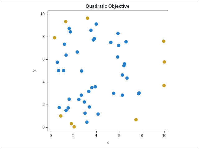
The selected points are along the border, but some pairs of points are close to each other. The following statements plot the second solution:

/* plot the second solution */
proc sort data=plotdata2;
   by Select;
run;
title 'Maxmin Objective';
proc sgplot data=plotdata2 aspect=1 noautolegend;
   scatter x=x y=y / group=Select;
run;

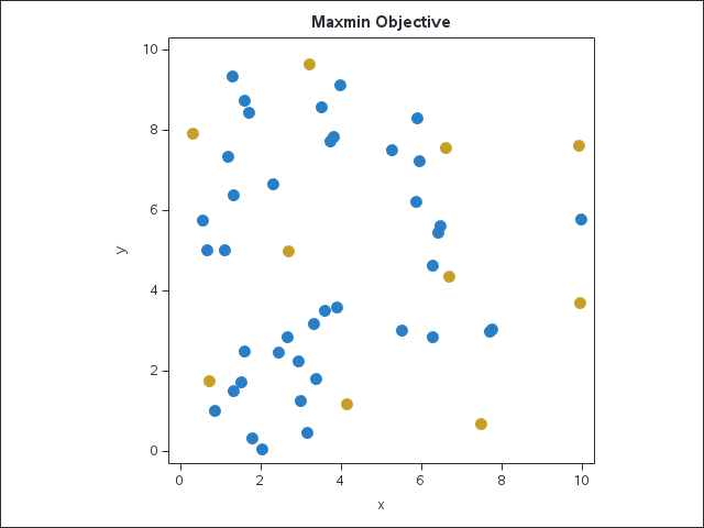
You can see that no two selected points are close to each other.

Conclusion

This example illustrates two of the automated linearization transformations (products of binary variables, and maximizing a minimum) that are now available in OPTMODEL just by adding the LINEARIZE keyword to the SOLVE statement. OPTMODEL introduces the required additional variables and constraints on your behalf and returns the optimal solution in terms of the original variables. Please try the other automated linearizations and let us know about any additional features that you would like to see introduced.

LEARN MORE | SAS Optimization