In my earlier blog, I described how to create maps in SAS Visual Analytics 8.2 if you have an ESRI shapefile with  granular geographies, such as counties, that you wish to combine into regions. Since posting this blog in January 2018, I received a lot of questions from users on a range of mapping topics, so I thought a more general post on using – and troubleshooting - custom polygons in SAS Visual Analytics on Viya was in order. Since version 8.3 is now generally available, this post is tailored to the 8.3 version of SAS Visual Analytics, but the custom polygon functionality hasn’t really changed between the 8.2 and 8.3 releases.

What are custom polygons?

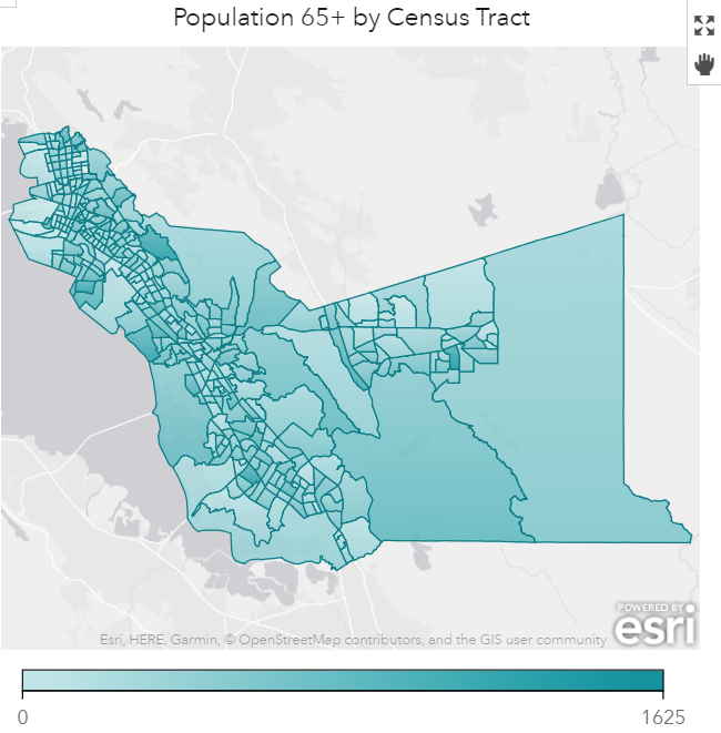
Custom polygons are geographic boundaries that enable you to visualize data as shaded areas on the map. They are also sometimes referred to as a choropleth maps. For example, you work for a non-profit organization which is trying to decide where to put a new senior center. So you create a map that shows the population of people over 65 years of age by US census tract. The darker polygons suggest a larger number of seniors, and thus a potentially better location to build a senior center:

SAS Visual Analytics 8.3 includes a few predefined polygonal shapes, including countries and states/provinces. But if you need something more granular, you can upload your own polygonal shapes.

How do I create my own polygonal shapes?

To create a polygonal map, you need two components:

1. A dataset with a measure variable and a region ID variable. For example, you may have population as a measure, and census tract ID as a region ID. A simple frequency can be used as a measure, too.
2. A “polygon provider” dataset, which contains the same region ID as above, plus geographic coordinates of each vertex in each polygon, a segment ID and a sequence number.

So where do I get this mysterious polygon provider? Typically, you will need to search for a shapefile that contains the polygons you need, and do a little bit of data preparation. Shapefile is a geographic data format supported by ESRI. When you download a shapefile and look at it on the file system, you will see that it contains several files. For example, my 2010 Census Tract shapefile includes all these components:

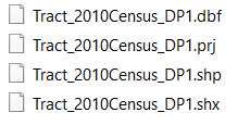
Sometimes you may see other components present as well. Make sure to keep all components together.

To prepare this data for SAS Visual Analytics, you have two options.

Preparing shapefile for SAS Visual Analytics: The long way

One method to prepare the polygon provider is to run PROC MAPIMPORT to convert the shapefile into a SAS dataset, add a sequence ID field and then load into the Cloud Analytic Services (CAS) server in SAS Viya. The sequence ID is mandatory, as it helps SAS Visual Analytics to draw the lines connecting vertices in the correct order.

A colleague recently reached out for help with a map of Census block groups for Chatham County in North Carolina. Let’s look at his example:

The shapefile was downloaded from here. We then ran the following code on my desktop:

libname geo 'C:\...\Data';
 
proc mapimport datafile="C:\...\Data\Chatham_County__2010_Census_Block_Groups.shp"
out=work.chatham_cbg;
run;
 
data geo.chatham_cbg;
set  chatham_cbg;
seqno=_n_;
run;

We then manually loaded the geo.chatham_cbg dataset in CAS using self-service import in SAS Visual Analytics. If you are not sure how to upload a dataset to CAS, please check the documentation.

Preparing shapefile for SAS Visual Analytics: %SHPIMPR macro shortcut

If the steps above seemed like a lot of work, you will be glad to know that all of this can be accomplished with a simple macro called %SHPIMPR. The macro will automatically run PROC MAPIMPORT, create a sequence ID variable and load the table into CAS. Here’s an example:

%shpimprt(shapefilepath=/path/Chatham_County__2010_Census_Block_Groups.shp, id=GEOID, outtable=Chatham_CBG, cashost=my_viya_host.com,   casport=5570, caslib='Public');

For this macro to work, the shapefile must be copied to a location that your SAS Viya server can access, and the code needs to be executed in an environment that has SAS Viya installed. So, it wouldn’t work if I tried to run it on my desktop, which only has SAS 9.4 installed. But it works beautifully if I run it in SAS Studio on my SAS Viya machine.

Configuring the polygon provider

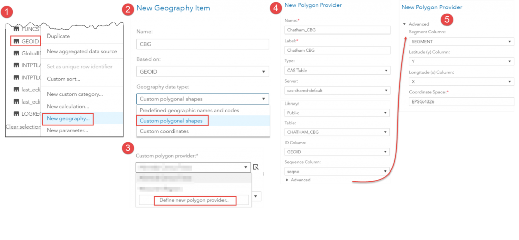
The next step is to configure the polygon provider inside your report. I provided a detailed description of this in my earlier blog, so here I’ll just summarize the steps:

• Add your data to the SAS Visual Analytics report, locate the region ID variable, right-click and select New Geography
• Give it a name and select Custom Polygonal Shapes as geography type
• Click on the Custom Polygon Provider box and select Define New Polygon Provider
• Configure your polygon provider by selecting the library, table and ID column. The values in your ID column must match the values of the region ID variable in the dataset you are visualizing. The ID column, however, does not need to have the same name as in the visualization dataset.
• If necessary, configure advanced options of the polygon provider (more on that in the troubleshooting section of this blog).

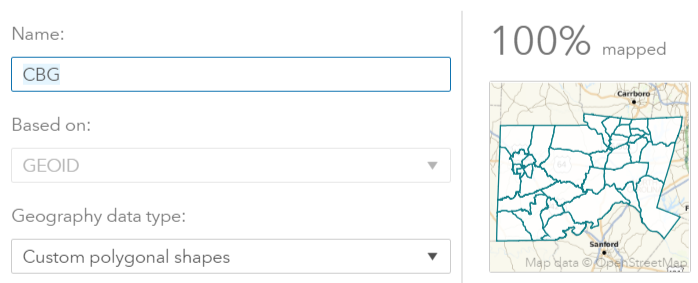
If all goes well, you should see a preview of your polygons and a percentage of regions mapped. Click OK to save your geographic item, and feel free to use it in the Geo Map object.

I followed your instructions, but the map is not working. What am I missing?

I observed a few common troubleshooting issues with custom maps, and all are fairly easy to fix. The table below summarizes symptoms and solutions.
 

Symptom		Solution
In the Geographic Item preview, 0% of the regions are mapped. For example: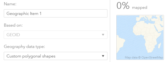		Check that the values in the region ID variable match between the main dataset and the polygon provider dataset.
I successfully created the map, but the colors of the polygons all look the same. I know I have a range of values, but the map doesn’t convey the differences.		In your main dataset, you probably have missing region ID values or region IDs that don’t exist in the polygon provider dataset. Add a filter to your Geo Map object to exclude region IDs that can’t be mapped.
Only a subset of regions is rendered.		You may have too many points (vertices) in your polygon provider dataset. SAS Visual Analytics can render up to 250,000 points. If you have a large number of polygons represented in a detailed way, you can easily exceed this limit. You have two options, which you can mix and match: (1)    Filter the map to show fewer polygons (2)    Reduce the level of detail in the polygon provider dataset using PROC GREDUCE. See example here. Also, if you imported data using the %shpimprt macro, it has an option to reduce the dataset. Here’s a handy link to documentation.
In the Geographic Item preview, the note shows that 100% of the regions are mapped, but the regions don’t render, or the regions are rendered in the wrong location (e.g., in the middle of the ocean) and/or at an incorrect scale.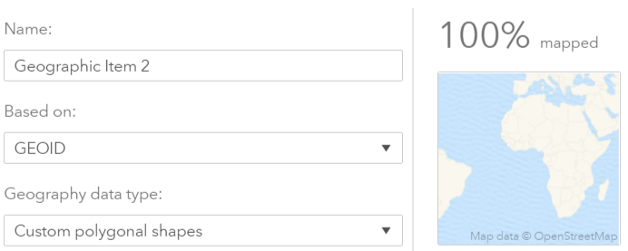		This is probably the trickiest issue, and the most likely culprit is an incorrectly specified coordinate space code (EPSG code). The EPSG code corresponds to the type of projection applied to the latitude and longitude in the polygon provider dataset (and the originating shapefile). Projection is a method of displaying points from a sphere (the Earth) on a two-dimensional plane (flat surface). See this tutorial if you want to know more about projections. 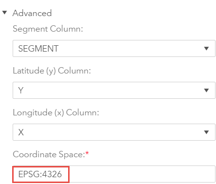There are several projection types and numerous flavors of each type. The default EPSG code used in SAS Visual Analytics is EPSG:4326, which corresponds to the unprojected coordinate system.  If you open advanced properties of your polygon provider, you can see the current EPSG code: Finding the correct EPSG code can be tricky, as not all shapefiles have consistent and reliable metadata built in. Here are a couple of things you can try: (1)    Open your shapefile as a layer in a mapping application such as ArcMap (licensed by ESRI) or QGIS (open source) and view the properties of the layer. In many cases the EPSG code will appear in the properties. (2)    Go to the location of your shapefile and open the .prj file in Notepad. It will show the projection information for your shapefile, although it may look a bit cryptic. Take note of the unit of measure (e.g., feet), datum (e.g., NAD 83) and projection type (e.g., Lambert Conformal Conic). Then, go to https://epsg.io/ and search for your geography.  Going back to the example for Chatham county, I searched for North Carolina. If more than one code is listed, select a few codes that seem to match your .prj information the best, then go back to SAS Visual Analytics and change the polygon provider Coordinate Space property. You may have to try a few codes before you find the one that works best.
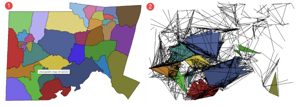
I ruled out a projection issue, the note in Geographic Item preview shows that 100% of the regions are mapped, but the regions still don’t render.		Take a look at your polygon provider preparation code and double-check that the order of observations didn’t accidentally get changed. The order of records may change, for example, if you use a PROC SQL join when you prepare the dataset. If you accidentally changed the order of the records prior to assigning the sequence ID, it can result in an illogical order of points which SAS Visual Analytics will have trouble rendering. Remember, sequence ID is needed so that SAS Visual Analytics can render the outlines of each polygon correctly. You can validate the order of records by mapping the polygon provider using PROC GMAP, for example: proc gmap map=geo.chatham_cbg data=geo.chatham_cbg; id geoid; choro geoid / nolegend levels=1; run; For example, in image #1 below, the records are ordered correctly. In image #2, the order or records is clearly wrong, hence the lines going crisscross.

 
As you can see, custom regional maps in SAS Visual Analytics 8.3 are pretty straightforward to implement. The few "gotchas" I described will help you troubleshoot some of the common issues you may encounter.

P.S. I would like to thank Falko Schulz for his help in reviewing this blog.