[Nabaruna Karmakar was coauthor of this post]

A study was conducted at the University of Denver on The Economic Impacts of the Austin, Texas "No Kill" Resolution. The study found great value in creating an animal welfare-focused community. It highlighted the benefits of economic growth due to an increased need in veterinary care, and the potential for attracting a like-minded, pet-loving workforce for companies located in Austin. The study also spoke about the costs associated with developing such a community – part of which included expenses related to staffing the animal shelters.

Like many non-profits, a shelter’s necessity to keep staffing costs low while scheduling enough employees to cover the demand during peak hours can be a struggle. In many organizations, managers often rely on personal judgment to create staff schedules, leading to higher labor costs in the case of overstaffing, or unmet needs in the case of understaffing.

In this article, we present a mixed integer linear programming (MILP) model to help an animal shelter create an optimal workforce schedule that meets the staffing demands at minimum cost.  With minor tweaks, the model could easily be adapted to many other non-profit or for-profit settings, such as scheduling bartenders, servers, and hosts in a restaurant, or scheduling nurses, nursing assistants, and administrative staff at a COVID-19 testing site.

Problem Description

We begin any optimization problem by identifying the three main components: the decisions we need to make, the goal we want to achieve by those decisions, and the constraints that prevent us from making certain decisions. We describe each of these next.

At this animal shelter, we have three types of employees: full-time employees, part-time employees, and volunteers. The animal shelter is open daily from 9 a.m. to 8 p.m. Therefore, our decisions are which employees should be scheduled during each hour of each day in a one-week time frame. Our goal (or objective) is to minimize the total labor cost, which includes regular wages and overtime wages for the full-time and part-time employees. The volunteers have no labor cost.

The constraints are what make the optimization problem interesting. Without constraints, our minimum labor cost would be zero, because we simply wouldn’t schedule any full-time or part-time employees. But we have a limited number of volunteers, and they are not qualified to perform every job at the shelter. Therefore, relying only on volunteers is not an acceptable solution because it leaves many needs unmet. In our problem, the schedule must satisfy the following constraints:

1. Full-time employees must be assigned either five or six shifts per week, with each shift being between eight and 10 consecutive hours.
2. Part-time employees must be assigned either five or six shifts per week, with each shift being between four and seven consecutive hours.
3. Volunteers can be scheduled for shifts of up to three consecutive hours, and they can specify the maximum number of days they are willing to volunteer in each week.
4. Full-time and part-time employees must receive overtime pay equal to 1.5 times their hourly wage for any hours worked beyond a specified threshold. For full-time employees, this threshold is 40 hours; for part-time employees, it is 20 hours.
5. Full-time and part-time employees should be given two consecutive days off unless they are assigned overtime, and volunteers should be given two consecutive days off. The employees and volunteers can specify which two days they would like to take off. If no preference is specified for some employees and volunteers, the model chooses two consecutive days off for these employees and volunteers.
6. The shelter has four different jobs that the employees and volunteers must perform: walking, feeding, administrative, and grooming. The schedule must satisfy the demand for each job in each hour of each day.
7. Employees and volunteers have different skill sets, which dictate the set of jobs each person can perform. We assume the jobs are nested, such that an employee who is qualified for one job is also qualified for all the jobs that require a lower skill level. Specifically:
   • An employee or volunteer who is qualified for grooming can also perform administrative jobs, feeding, and walking.
   • An employee or volunteer who is qualified for administrative jobs can also perform feeding and walking.
   • An employee or volunteer who is qualified for feeding can also perform walking.
   • An employee or volunteer who is qualified only for walking cannot perform any other jobs.

Input Data Overview

Before we describe the mathematical formulation for this optimization problem, let's take a look at the input data in order to better understand the decisions, objective, and constraints described in the previous section. The input data include an Employees table, a Jobs table, a Demand table, and a Demand Coefficients table.

Employees Table and Jobs Table

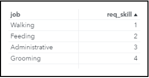
The Employees table contains the full employee and volunteer roster, consisting of 16 full-time employees, 15 part-time employees, and 10 volunteers. A portion of the table is shown in Figure 1. The skill column identifies the employee’s skill level; the numeric values {1, 2, 3, 4} are mapped to the jobs of {Walking, Feeding, Administrative, Grooming} in the Jobs table shown in Figure 2.

The cost column in the Employees table contains the hourly wage for each employee; note that the hourly wage for volunteers is always zero. In the off_days column, you can see that some employees and volunteers have specified which two consecutive days they would like to receive off, but other employees and volunteers have not indicated a preference and will let the scheduler decide. Finally, the max_volunteer_days column indicates the maximum number of days that a volunteer is willing to work each week. In our data, volunteers are willing to work either two or three days per week.

Demand Table and Demand Coefficients Table

The Demand table shown in Figure 3 contains a prediction of the number of animals that will be in the animal shelter during each hour of each day of the week; col9 represents the predicted number of animals at 9 a.m., col10 represents the predicted number of animals at 10 a.m., and so on. We calculate the demand for the four jobs (Walking, Feeding, Administrative, and Grooming) as a proportion of the expected number of animals in the shelter, and the Demand Coefficients table shown in Figure 4 contains the multipliers that are used to calculate the demand for each job at each time. Note that the demand coefficients do not vary by day of the week, but they do vary by time. For example, feeding happens only between 9 a.m. and noon, and again between 5 p.m. and 8 p.m.

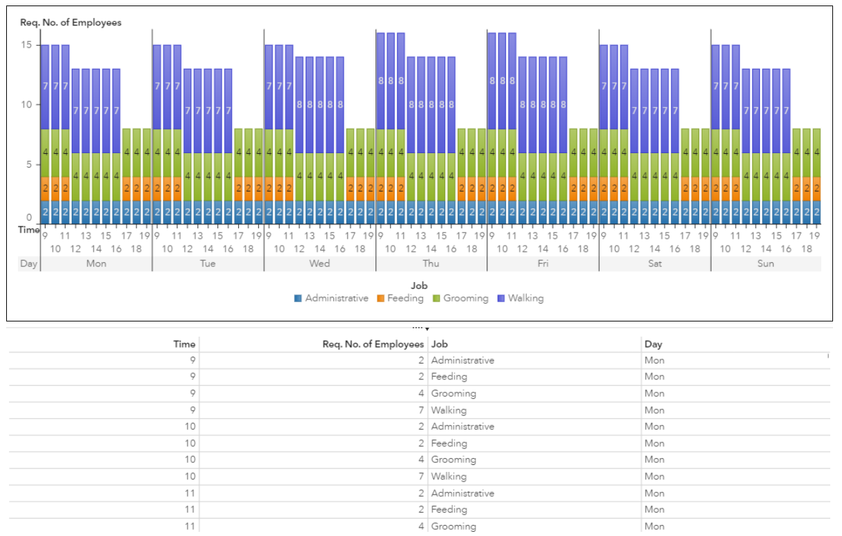
The bar chart and accompanying detail table in Figure 5 show the number of employees required to cover each job throughout the week, calculated using both the predicted demand from the Demand table and the job demand coefficients from the Demand Coefficients table.

Model Formulation

We use the runOptmodel CAS action in SAS Optimization to model and solve this optimization problem, so we begin our code with a call to PROC CAS followed by a SOURCE statement that enables us to assign the OPTMODEL statements that follow to a variable called pgm. Then we declare the index sets and parameters that we use to store the data for the problem, and we use READ DATA statements to read the four input tables and populate the index sets and parameters.

proc cas; 
source pgm;
 
   num first_hour = 9;
   num last_hour = 19;
   set <str> EMPLOYEES;
   set <str> DAYS;
   set <str> JOBS;
   set TIMES={first_hour..last_hour};
 
   num demand{DAYS, TIMES};
   num demand_coef{JOBS, TIMES};
   num req_skill{JOBS};
   num base_cost init 1;
   num over_cost init 1.5;
 
   num skill{EMPLOYEES};
   num cost{EMPLOYEES};
   num min_shift{EMPLOYEES};
   num max_shift{EMPLOYEES};
   num min_hour{EMPLOYEES};
   num max_hour{EMPLOYEES};
   num max_volunteer_days{EMPLOYEES};
   str type{EMPLOYEES};
   str off_days{EMPLOYEES};
 
   read data casuser.ASO_employees 
      into EMPLOYEES=[id] skill type cost off_days max_volunteer_days;
 
   read data casuser.ASO_jobs 
      into JOBS=[job] req_skill;
 
   read data casuser.ASO_demand
      into DAYS=[day] {t in TIMES} <demand[day,t]= col('col'||t)>;
 
   read data casuser.ASO_demand_coef
      into [job time] demand_coef;

Next we construct some additional derived sets that are helpful in modeling the problem. For each employee, we create the following derived sets:

• QUALIFIED_JOBS: The set of jobs that the employee is qualified to perform.
• EMPLOYEE_REGULAR_DAYS: The set of days that the employee has not specifically requested to take off.
• EMPLOYEE_OT_DAYS: The set of days that the employee could potentially be assigned an overtime shift. For volunteers, this is an empty set because volunteers are not allowed to work overtime. For part-time and full-time employees, the set depends on whether the employee has requested specific days off. If an employee has requested specific days off, then EMPLOYEE_OT_DAYS contains the requested days off; if an employee is assigned to work on any of these days, it must be an overtime shift. If an employee has not requested specific days off, then EMPLOYEE_OT_DAYS contains the set of all days because any day is a potential overtime day if the employee exceeds the number of regular time shifts.
• EMPLOYEE_DAYS: The set of days that an employee is eligible to work. This is simply the union of EMPLOYEE_REGULAR_DAYS and EMPLOYEE_OT_DAYS. For part-time and full-time employees, this is the same as the set DAYS, but for volunteers it excludes any days that the volunteer has specifically requested to take off.

   set QUALIFIED_JOBS{i in EMPLOYEES} = {j in JOBS: skill[i] >= req_skill[j]};
 
   set EMPLOYEE_REGULAR_DAYS{i in EMPLOYEES} = DAYS diff {scan(off_days[i],1,'-')} diff {scan(off_days[i],2,'-')};
 
   set EMPLOYEE_OT_DAYS{i in EMPLOYEES} = if type[i]='Volunteer' then {} 
                                          else (if missing(off_days[i]) then DAYS 
                                                else DAYS diff EMPLOYEE_REGULAR_DAYS[i]);
 
   set EMPLOYEE_DAYS{i in EMPLOYEES} = EMPLOYEE_REGULAR_DAYS[i] union EMPLOYEE_OT_DAYS[i];

The next section of the code populates some parameters with the hard-coded values we are using for the minimum and maximum number of shifts and length of shifts for each type of employee. We could have included additional columns in the Employees table and added these columns to the READ DATA statement to populate the parameters, and the employees could have had different values for the minimum and maximum number of shifts and number of hours per shift. However, since we are assuming constant values for all employees within each employee type, we are populating the values directly within the OPTMODEL code. The COALESCE function means that if a Volunteer has a missing value for max_volunteer_days, we are assigning a default value of 3.

We also create a parameter called next_day that stores the string corresponding to the next day of the week for each day. We use this parameter to ensure that employees get two consecutive days off even when they haven't requested specific days off.

   for {i in EMPLOYEES} do;
      if type[i] = 'Full-Time' then do;
         min_shift[i] = 5;
         max_shift[i] = 6;
         min_hour[i] = 8;
         max_hour[i] = 10;
      end;
      else if type[i] = 'Part-Time' then do;
         min_shift[i] = 5;
         max_shift[i] = 6;
         min_hour[i] = 4;
         max_hour[i] = 7;
      end;
      else if type[i] = 'Volunteer' then do;
         min_shift[i] = 0;
         max_shift[i] = coalesce(max_volunteer_days[i],3);
         min_hour[i] = 0;
         max_hour[i] = 3;
      end;
   end;
 
   str next_day{DAYS};
   for {d in DAYS} do;
      if      d = 'Mon' then next_day[d] = 'Tue';
      else if d = 'Tue' then next_day[d] = 'Wed';
      else if d = 'Wed' then next_day[d] = 'Thu';
      else if d = 'Thu' then next_day[d] = 'Fri';
      else if d = 'Fri' then next_day[d] = 'Sat';
      else if d = 'Sat' then next_day[d] = 'Sun';
      else if d = 'Sun' then next_day[d] = 'Mon';
   end;

The main decision variables in this problem are Assign_To_Job[i,j,t,d], and they are binary variables. Assign_To_Job[i,j,t,d] has a value of 1 if employee i is assigned to job j at time t on day d, and it has a value of 0 otherwise. If we know the values of these decision variables, we have everything we need to construct the employee schedule and determine the associated cost. However, the model needs some additional auxiliary variables to force relationships in the constraints; for example, to make sure that each employee satisfies the minimum and maximum number of shifts.

The additional variables are also binary. For example, Assign_To_Regular_Day[i,d] has a value of 1 if employee i is assigned to work a regular shift on day d, and it has a value of 0 otherwise. Likewise, Assign_To_Overtime_Day[i,d] has a value of 1 if employee i is assigned to work an overtime shift on day d, and it has a value of 0 otherwise.

Note that the variables Is_Working_Hour and Is_Working_Day could have been modeled as implicit variables by using the IMPVAR statement instead of the VAR statement. Is_Working_Hour[i,t,d] is simply the sum of Assign_To_Job[i,j,t,d] over all qualified jobs j, and Is_Working_Day[i,d] is simply the sum of Assign_To_Regular_Day[i,d] and Assign_To_Overtime_Day[i,d]. We tested both formulations, and for this particular problem, modeling them as explicit variables resulted in a slight improvement in the run time. In general, the explicit variable formulation can reduce the number of constraint coefficients when the variable appears in several places, but it will not always result in faster performance. You should experiment with both formulations in your models if run-time performance is a primary concern.

We use the variables called Two_Days_Off_Start_Day to indicate the first day off in a consecutive two-day period. For example, if Two_Days_Off_Start_Day[i,'Mon'] = 1, it means that employee i is not scheduled on Monday or Tuesday as a regular day. These variables are defined only for employees who did not request specific days off and whose maximum number of shifts per week is greater than three. If an employee works three or fewer days in the week, we know that the employee must already receive at least two consecutive days off. In our problem instance, this is the case only for volunteers.

The Switch variables are needed to make sure that employees work consecutive hours during a shift. For example, if a full-time employee is scheduled for eight hours on Monday, we would not want those hours to be 8 a.m. to 9 a.m., then 11 a.m. to 1 p.m., then 2 p.m. to 4 p.m., then 5 p.m. to 8 p.m. The Switch variables will be explained in more detail when we get to the corresponding constraints.

Finally, we can fix the values of some variables for decisions that we already know must be true. Full-time and part-time employees must work a minimum of five days. If an employee has requested two specific days off, then we know which five days must be worked as regular shifts before any overtime shifts can be assigned to the employee on one of the requested days off. In general, if the number of regular days available for an employee is equal to the minimum number of days the employee must work, then we know the employee must be assigned to work on each available regular day. Therefore, we can fix both Assign_To_Regular_Day[i,d] and Is_Working_Day[i,d] to 1 for these days.

   /******************************** Variables *******************************/
 
   var Assign_To_Job {i in EMPLOYEES, QUALIFIED_JOBS[i], TIMES, EMPLOYEE_DAYS[i]} binary;
 
   var Assign_To_Regular_Day {i in EMPLOYEES, EMPLOYEE_REGULAR_DAYS[i]} binary;
   var Assign_To_Overtime_Day {i in EMPLOYEES, EMPLOYEE_OT_DAYS[i]} binary;
 
   var Is_Working_Hour {i in EMPLOYEES, TIMES, EMPLOYEE_DAYS[i]} binary;
   var Is_Working_Day {i in EMPLOYEES, EMPLOYEE_DAYS[i]} binary;
 
   var Two_Days_Off_Start_Day {i in EMPLOYEES, DAYS: missing(off_days[i]) and max_shift[i] > 3} binary;
 
   var Switch {i in EMPLOYEES, TIMES, EMPLOYEE_DAYS[i]} binary;
 
   for {i in EMPLOYEES: card(EMPLOYEE_REGULAR_DAYS[i])=min_shift[i]} do;
      for {d in EMPLOYEE_REGULAR_DAYS[i]} do;
         fix Assign_To_Regular_Day[i,d] = 1;
         fix Is_Working_Day[i,d] = 1;
      end;
   end;

The objective is to minimize the total cost, which consists of a base cost and an overtime cost. Notice that we are calculating the overtime cost as only the additional premium beyond an employee's regular hourly wage. For example, suppose a full-time employee with an hourly wage of $20 works 48 hours in the week. We are considering the base cost to be $20 * 48, and the overtime cost to be $10 * 8. In some situations, you might want to instead consider the base cost to be $20 * 40 and the overtime cost to be $30 * 8. Since we are minimizing the total cost, both interpretations of overtime cost are equivalent in terms of the objective, and we have chosen the former interpretation because it simplifies the model. If you want to report base and overtime costs differently in the solution, a simple postprocessing step after the SOLVE statement could be used to calculate different costs per employee.

   /******************************** Objective *******************************/
 
   min BaseCost
      = base_cost * sum{i in EMPLOYEES, t in TIMES, d in EMPLOYEE_DAYS[i]} cost[i] * Is_Working_Hour[i,t,d];
 
   min OverTimeCost
      = (over_cost - base_cost) * sum {i in EMPLOYEES} 
                                       cost[i] * (sum {t in TIMES, d in EMPLOYEE_DAYS[i]} Is_Working_Hour[i,t,d] 
                                                  - min_shift[i] * min_hour[i]);
 
   min TotalCost
      = BaseCost + OverTimeCost;

Before we move on to the constraints, we first need to say a word about DECOMP. Most of our constraints are applied individually to each employee, and the only constraints that span multiple employees are the demand satisfaction constraints. Therefore, this problem's structure is a natural fit for using a decomposition algorithm. When we define the constraints, we use a constraint suffix to identify each constraint with a particular decomposition block. First, however, we need to define the blocks. We have chosen to define the blocks according to each employee/day pair. We tested blocks at the employee level and at employee/day level and we saw slightly better performance from the employee/day level. In your applications, you might want to experiment with different block assignments to find the one that works best. If you don't know what your blocks should be, you can still use the DECOMP algorithm, which first attempts to identify suitable blocks. But because we already know something about the structure of the constraints, it is helpful to identify them to the DECOMP algorithm. Here we are simply creating a unique numeric index called block_id[i,d] for each [i,d] pair.

   /****************************** Blocks Setup ******************************/
   num block_id{EMPLOYEES, DAYS};
   num id init 0;
   for {i in EMPLOYEES, d in DAYS} do;
      block_id[i,d] = id;
      id = id + 1;
   end;

Next we describe the constraints. The first few constraints are fairly intuitive. Is_Working_Hour and Is_Working_Day are the variables that we chose to model as explicit variables rather than implicit variables for a slight boost in performance, and the corresponding constraints simply define the relationship between these variables and the other binary variables.

The Satisfy_Demand constraint ensures that we schedule enough employees to cover the requirements for each job during each time period on each day. Assign_Day_If_Assign_Job is a linking constraint that ensures that if an employee is working during any time period of a day, the employee is considered to be working on that day.

Note the suffixes=(block=block_id[i,d]) option at the end of each of these constraints except the Satisfy_Demand constraint. This is how we identify a constraint with a particular block to be used in the decomposition algorithm—we assign to the block keyword the unique numeric index block_id[i,d] that we created in a previous step. We cannot include this suffix on the Satisfy_Demand constraint because it spans multiple employees, but the other constraints are applied individually to each employee/day pair and therefore can be assigned to the DECOMP blocks.

   /******************************* Constraints ******************************/
 
   con Define_Is_Working_Hour {i in EMPLOYEES, t in TIMES, d in EMPLOYEE_DAYS[i]}:
      Is_Working_Hour[i,t,d] = sum{j in QUALIFIED_JOBS[i]} Assign_To_Job[i,j,t,d]
         suffixes=(block=block_id[i,d]);
 
   con Define_Is_Working_Day {i in EMPLOYEES, d in EMPLOYEE_DAYS[i]}:
      Is_Working_Day[i,d] = (if d in EMPLOYEE_REGULAR_DAYS[i] then Assign_To_Regular_Day[i,d]) 
                          + (if d in EMPLOYEE_OT_DAYS[i] then Assign_To_Overtime_Day[i,d])
         suffixes=(block=block_id[i,d]);
 
   con Satisfy_Demand {j in JOBS, t in TIMES, d in DAYS}:
      sum {i in EMPLOYEES: j in QUALIFIED_JOBS[i] and d in EMPLOYEE_DAYS[i]} Assign_To_Job[i,j,t,d] 
      >= demand_coef[j,t] * demand[d,t];
 
   con Assign_Day_If_Assign_Job {i in EMPLOYEES, j in QUALIFIED_JOBS[i], t in TIMES, d in EMPLOYEE_DAYS[i]}:
      Is_Working_Day[i,d] >= Assign_To_Job[i,j,t,d]
         suffixes=(block=block_id[i,d]);

The next constraints enforce the minimum and maximum number of shifts (that is, days) per employee, and the minimum and maximum number of hours per shift. Note that Min_Num_Shifts uses the Assign_To_Regular_Day variables, while Max_Num_Shifts uses Is_Working_Day. This is because we want to include the possibility of overtime shifts in the maximum, but we only want to assign an overtime day if the employee has already been assigned the minimum number of shifts for regular time. Also note that we cannot use the suffixes=(block=block_id[i,d]) option on the Min_Num_Shifts and Max_Num_Shifts constraints. Even though these constraints are applied individually for each employee, they span multiple days, and we have defined our decomposition blocks according to employee/day pairs.

   con Min_Num_Shifts {i in EMPLOYEES: min_shift[i] > 0}:
      sum {d in EMPLOYEE_REGULAR_DAYS[i]} Assign_To_Regular_Day[i,d] >= min_shift[i];
 
   con Max_Num_Shifts {i in EMPLOYEES}:
      sum{d in EMPLOYEE_DAYS[i]} Is_Working_Day[i,d] <= max_shift[i]; 
 
   con Min_Hours_Per_Shift {i in EMPLOYEES, d in EMPLOYEE_DAYS[i]: min_hour[i] > 0}:
      sum {t in TIMES} Is_Working_Hour[i,t,d] >= min_hour[i] * Is_Working_Day[i,d]
         suffixes=(block=block_id[i,d]);
 
   con Max_Hours_Per_Shift {i in EMPLOYEES, d in EMPLOYEE_DAYS[i]}:
      sum {t in TIMES} Is_Working_Hour[i,t,d] <= max_hour[i]
         suffixes=(block=block_id[i,d]);

The next three constraints are a bit more complicated than the previous constraints. We need to force the hours that an employee works in a day to be consecutive, and for this we use the Switch variables. We are defining Switch[i,t,d] to have a value of 1 if employee i is not working in time t and begins working in time t+1 on day d, and 0 otherwise. We need to create constraints that force Switch to follow this definition, and then we can force Switch[i,t,d] to take a value of 1 for at most one time period t. In other words, we have at most one "switch" from non-working to working on a given day. The comments in the following section of code describe the conditions that we are forcing with each constraint; you can substitute different combinations of values of 0 and 1 for the other variables to understand how Switch[i,t,d] must behave in each case.

   /* If employee is not working in time t but working in time t+1, force Switch[i,t,d] to be 1. */
   con Force_Switch_to_1 {i in EMPLOYEES, t in TIMES, d in EMPLOYEE_DAYS[i]: t+1 <= last_hour}: 
      Is_Working_Hour[i,t,d] + Switch[i,t,d] >= Is_Working_Hour[i,t+1,d]
         suffixes=(block=block_id[i,d]);
 
   /* If employee is working in time t and also working in time t+1, force Switch[i,t,d] to be 0. 
      If employee is not working in time t and also not working in time t+1, force Switch[i,t,d] to be 0.
      If employee is working in time t and not working in time t+1, force Switch[i,t,d] to be 0. */
   con Force_Switch_to_0 {i in EMPLOYEES, t in TIMES, d in EMPLOYEE_DAYS[i]: t+1 <= last_hour}:
      Is_Working_Hour[i,t,d] + 2 * Switch[i,t,d] <= 1 + Is_Working_Hour[i,t+1,d]
         suffixes=(block=block_id[i,d]);
 
   /* Allow at most one switch per day. But if the employee begins work in the first hour, don't allow 
      any switches. */
   con Max_One_Switch_Per_Day {i in EMPLOYEES, d in EMPLOYEE_DAYS[i]}:
      sum{t in TIMES: t+1 <= last_hour} Switch[i,t,d] <= 1 - Is_Working_Hour[i,first_hour,d] 
         suffixes=(block=block_id[i,d]);

Finally, we need to add constraints to make sure that the employees who did request specific days off do get two consecutive days off unless they are assigned overtime. Recall that the binary variable called Two_Days_Off_Start_Day[i,d] has a value of 1 if day d is the first of two consecutive days off for employee d, and 0 otherwise. The first constraint below forces Two_Days_Off_Start_Day to have a value of 0 if either of the two days is assigned as a regular day, and the second constraint forces us to choose at least one day d with Two_Days_Off_Start_day[i,d] = 1. We only need to apply these constraints to the set of employees who did not request specific days off and who can work more than three days per week. If an employee can only work three or fewer days per week, then we know the employee is already receiving two consecutive days off.

   con Two_Days_Off_Zero_if_Working {i in EMPLOYEES, d in DAYS: missing(off_days[i]) and max_shift[i] > 3}:
      Assign_To_Regular_Day[i,d] + Assign_To_Regular_Day[i,next_day[d]] + 2*Two_Days_Off_Start_Day[i,d] <= 2; 
 
   con Force_Two_Days_Off {i in EMPLOYEES: missing(off_days[i]) and max_shift[i] > 3}:
      sum{d in DAYS} Two_Days_Off_Start_Day[i,d] >= 1;

Solving the Problem

After doing the work of modeling this optimization problem, solving it is the easy part! We are using the MILP solver to minimize the TotalCost objective. We have specified a maximum time of 300 seconds. Although this problem solves very quickly in under 30 seconds, it is a good practice to include a time bound in case we decide to modify the problem formulation in the future to accommodate additional constraints or to try different solver options. We are also specifying a relative objective gap of 0.1%.

We are using the DECOMP algorithm, and we specify HYBRID=FALSE so the root node processing is handled entirely by the decomposition algorithm, instead of first processing the root node using standard MILP techniques. Recall that we added the suffixes=(block=block_id[i,d]) option to the decomposable constraints in order to identify the block for each constraint. When blocks are defined, the default DECOMP option is METHOD=USER, so we do not need to specify it as an option in the SOLVE statement.

   /********************************** Solve *********************************/
 
   solve obj TotalCost with milp / maxtime=300 relobjgap=0.001 decomp=(hybrid=false);

After we solve the problem, we calculate the weekly base cost and overtime cost for each employee, and we use CREATE DATA statements to create output tables containing the job assignments and the employee costs.

   /****************************** Create Output *****************************/
 
   num regCost{EMPLOYEES}, OTCost{EMPLOYEES} init 0;
   for {i in EMPLOYEES} do;
      regCost[i] = base_cost * cost[i] * sum {t in TIMES, d in EMPLOYEE_DAYS[i]} 
                                               round(Is_Working_Hour[i,t,d].sol,1);
      OTcost[i] = (over_cost - base_cost) * cost[i] 
                   * (sum {t in TIMES, d in EMPLOYEE_DAYS[i]} round(Is_Working_Hour[i,t,d].sol,1) 
                      - min_shift[i] * min_hour[i]);
   end;
 
   create data casuser.job_assignments
      from [employee job time day] = {i in EMPLOYEES, j in QUALIFIED_JOBS[i], t in TIMES, d in EMPLOYEE_DAYS[i]:
                                      Assign_To_Job[i,j,t,d].sol > 0.9};
 
   create data casuser.employee_costs
      from [employee] = {i in EMPLOYEES}
         base_cost = regCost[i]
         overtime_cost = OTcost[i];

As the last step in our code, we need to use an ENDSOURCE statement to terminate the block of code that is stored in the pgm variable. Then we use the ACTION statement to call the runOptmodel CAS action from the optimization action set, and we use code=pgm to pass the OPTMODEL statements to the runOptmodel action.

endsource;
 
    action optimization.runOptmodel / code=pgm printlevel=2; run; 
 
quit;

Optimization Log and Output Tables

The optimization log is shown below. It first describes the problem structure, including the numbers of variables and constraints both before and after the presolver step. Next you can see information about the DECOMP algorithm, such as the number of blocks (275) and the decomposition subproblem coverage (approximately 97% of variables and 95% of constraints). Finally, the iteration log shows information about each iteration until we reach the convergence criteria. The optimal total cost for our problem is $22,010.

NOTE: Active Session now MYCASSESSION.
NOTE: There were 41 rows read from table 'ASO_EMPLOYEES' in caslib 'CASUSER'.
NOTE: There were 4 rows read from table 'ASO_JOBS' in caslib 'CASUSER'.
NOTE: There were 7 rows read from table 'ASO_DEMAND' in caslib 'CASUSER'.
NOTE: There were 44 rows read from table 'ASO_DEMAND_COEF' in caslib 'CASUSER'.
NOTE: Problem generation will use 16 threads.
NOTE: The problem has 14957 variables (0 free, 210 fixed).
NOTE: The problem uses 2 implicit variables.
NOTE: The problem has 14957 binary and 0 integer variables.
NOTE: The problem has 18244 linear constraints (3411 LE, 3300 EQ, 11533 GE, 0 range).
NOTE: The problem has 62397 linear constraint coefficients.
NOTE: The problem has 0 nonlinear constraints (0 LE, 0 EQ, 0 GE, 0 range).
NOTE: The remaining solution time after problem generation and solver initialization is 299.65 seconds.
NOTE: The initial MILP heuristics are applied.
NOTE: The MILP presolver value AUTOMATIC is applied.
NOTE: The MILP presolver removed 5994 variables and 11044 constraints.
NOTE: The MILP presolver removed 31843 constraint coefficients.
NOTE: The MILP presolver added 2827 constraint coefficients.
NOTE: The MILP presolver modified 723 constraint coefficients.
NOTE: The presolved problem has 8963 variables, 7200 constraints, and 30554 constraint coefficients.
NOTE: The MILP solver is called.
NOTE: The Decomposition algorithm is used.
NOTE: The Decomposition algorithm is executing in single-machine mode.
NOTE: The DECOMP method value USER is applied.
NOTE: The problem has a decomposable structure with 275 blocks. The largest block covers 0.5556% of the constraints in the problem.
NOTE: The decomposition subproblems cover 8718 (97.27%) variables and 6817 (94.68%) constraints.
NOTE: The deterministic parallel mode is enabled.
NOTE: The Decomposition algorithm is using up to 16 threads.
      Iter         Best       Master         Best       LP       IP  CPU Real
                  Bound    Objective      Integer      Gap      Gap Time Time
NOTE: Starting phase 1.
         1       0.0000     589.0000            . 5.89e+02        .    4    3
        10       0.0000      14.5333            . 1.45e+01        .    5    4
        17       0.0000       0.0000            .    0.01%        .    6    4
        18       0.0000       0.0000            .    0.00%        .    6    4
NOTE: Starting phase 2.
        19   14510.0000   30203.5804            .  108.16%        .    7    5
        20   14510.0000   26027.3000   24617.0000   79.37%   69.66%   11    8
        26   14510.0000   23147.0000   23546.0000   59.52%   62.27%   14   10
        28   15701.9000   22998.5000   23457.5000   46.47%   49.39%   14   10
        30   15701.9000   22900.2500   23214.5000   45.84%   47.85%   14   11
        33   15701.9000   22697.5000   23133.5000   44.55%   47.33%   15   11
        35   15701.9000   22593.5000   23091.5000   43.89%   47.06%   15   11
        38   15701.9000   22541.5000   23046.5000   43.56%   46.78%   16   11
        40   15701.9000   22457.0000   22479.5000   43.02%   43.16%   18   14
        43   15701.9000   22422.5000   22472.0000   42.80%   43.12%   19   14
        46   21627.5000   22422.5000   22442.0000    3.68%    3.77%   19   14
        50   21627.5000   22415.0000   22359.5000    3.64%    3.38%   19   15
        52   21627.5000   22229.5000   22287.5000    2.78%    3.05%   20   15
        54   21627.5000   22182.5000   22251.5000    2.57%    2.89%   20   15
        59   21627.5000   22010.0000   22118.0000    1.77%    2.27%   20   15
        60   22010.0000   22010.0000   22118.0000    0.00%    0.49%   20   15
         .   22010.0000   22010.0000   22118.0000    0.00%    0.49%   21   16
NOTE: Starting branch and bound.
         Node  Active   Sols         Best         Best      Gap    CPU   Real
                                  Integer        Bound            Time   Time
            0       1     26   22118.0000   22010.0000    0.49%     21     16
            7       9     27   22091.0000   22010.0000    0.37%     44     27
            8       0     29   22010.0000   22010.0000    0.00%     44     27
NOTE: The Decomposition algorithm used 16 threads.
NOTE: The Decomposition algorithm time is 27.87 seconds.
NOTE: Optimal.
NOTE: Objective = 22010.
NOTE: The output table 'JOB_ASSIGNMENTS' in caslib 'CASUSER' has 1043 rows and 4 columns.
NOTE: The output table 'EMPLOYEE_COSTS' in caslib 'CASUSER' has 41 rows and 3 columns.
{,,,,,,,status=OK,algorithm=DECOMP,solutionStatus=OPTIMAL,objective=22010,numIterations=223,
presolveTime=1.9837138653,solutionTime=27.870479107,numSolutions=29,primalInf=4.440892E-16,
boundInf=4.440892E-16,bestBound=22010,numNodes=9,relObjGap=0,absObjGap=0,integerInf=4.440892E-16}

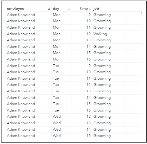
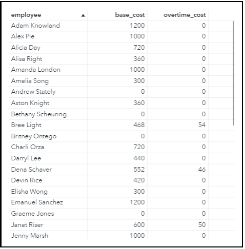
Figure 6 shows a portion of the output table called JOB_ASSIGNMENTS, and Figure 7 shows a portion of the output table called EMPLOYEE_COSTS. In these tables, we have everything we need to create an employee schedule for the week and to calculate the resulting wage costs. However, it is often useful to analyze the solution visually, which we do next.

Visualizing the Output

Now let's take a look at some helpful reports to visualize the output from the optimization model. The runOptmodel action produced the tabular output tables that were shown in Figure 6 and Figure 7. We used SAS Visual Analytics to analyze these tables with user-friendly visual representations.

Employee Schedule

Figure 8 shows a heat map displaying the assignment of the full-time employees on each day of the week marked by the green boxes. We can see that all full-time employees except Morgan Sound have been given two consecutive days off. The assigned days off are a mix of those provided as input by the user for the full-time employees that requested specific days off, or a decision by the model for the full-time employees who did not request specific days off. Morgan Sound requested Wednesday and Thursday off, but the optimization model has assigned him to work overtime on Thursday, so he receives only one day off.

Figure 9 shows a similar heat map for the part-time employees. We can see that five part-time employees work an additional overtime day and receive only one day off, while the remaining part-time employees receive two consecutive days off. Again, the assigned days off are a mix of those provided as input by the user for the part-time employees that requested specific days off, or a decision by the model for the part-time employees who did not request specific days off.

The weekly schedule of the volunteers is shown in Figure 10. The number of shifts assigned varies according to the max_volunteer_days input provided for each volunteer.

Overtime Analysis

The bar chart in Figure 11 shows the total cost for each full-time employee. The green portion of the bars represents regular wages, while the red portion represents overtime pay. We can see that Morgan Sound is receiving overtime pay for the extra shift that was assigned to him during the week. None of the other full-time employees receive overtime pay, which means that in addition to not working extra shifts, they are not assigned to work any additional hours for their regular shifts.

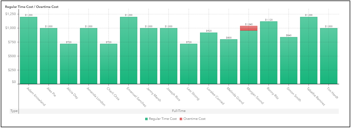
Figure 12 shows a similar chart for the part-time employees. The five part-time employees who were assigned an additional shift are all receiving overtime pay. Similar to the full-time employees, none of the other part-time employees receive overtime pay, which means that in addition to not working extra shifts, they are not assigned to work any additional hours for their regular shifts.

Summary

In this article, we showed a useful application of using the runOptmodel action in SAS Optimization to determine an optimal employee schedule at an animal shelter, and we used SAS Visual Analytics to create user-friendly reports to analyze the optimal solution. OPTMODEL separates the model from the data, and this enables the same model to be used for different problem instances simply by changing the input data tables. For example, if an employee decides to switch from full-time to part-time, or if some employees want to change their days off, or if any employees receive a pay raise, the model can easily handle the changes in the input data and provide a new optimal schedule.

Acknowledgments

The authors would like to thank Rob Pratt and Hossein Tohidi for their contributions to the model formulation.

Code