In the traveling salesman problem (TSP), a salesman must minimize travel distance while visiting each of a given set of cities exactly once. Recently, the TSP has generated some buzz in the popular media, after a blog post by Randy Olson. The tour shown was not quite optimal, and Bill Cook followed up with a very thorough discussion of the problem and an optimal tour. I'm pleased to report that you can solve this problem by using just a few lines of SAS code, in particular a SAS DATA step and the OPTNET procedure in SAS/OR:

filename myurl url 'http://www.math.uwaterloo.ca/tsp/usa50/europe50.tsp';
 
data indata;
   infile myurl firstobs=10;
   do i = 1 to 50;
      do j = 1 to i;
         input d @@;
         if i ne j then output;
      end;
   end;
run;
 
proc optnet data_links=indata;
   data_links_var from=i to=j weight=d;
   tsp;
run;

The resulting log shows that an optimal tour is found immediately (and proved to be optimal):

NOTE: The number of nodes in the input graph is 50.
NOTE: The number of links in the input graph is 1225.
NOTE: Processing the traveling salesman problem.
NOTE: The initial TSP heuristics found a tour with cost 22015038 using 0.09 
      (cpu: 0.06) seconds.
NOTE: The MILP presolver value NONE is applied.
NOTE: The MILP solver is called.
NOTE: The MILP solver added 11 cuts with 2927 cut coefficients at the root.
NOTE: Optimal.
NOTE: Objective = 22015038.
NOTE: Processing the traveling salesman problem used 0.10 (cpu: 0.06) seconds.

proc optmodel;
   set <num,num> EDGES;
   num d {EDGES};
   read data indata into EDGES=[i j] d;
   solve with network / tsp links=(weight=d);
quit;

In this blog post, I'll discuss a difficult variant of the TSP, namely the traveling baseball fan problem. The topic is timely because Sunday is April 5, Opening Day of the 2015 Major League Baseball regular season. I'm not really a baseball fan, but I am a fan of interesting optimization problems, especially difficult ones that can be attacked in more than one way. A few years ago, Phil Gibbs in SAS Technical Support mentioned this problem to me, and I was hooked. Tonya Chapman, Matthew Galati, and I wrote a SAS Global Forum paper on it last year. You can find the full paper here, so I'll just point out the highlights to motivate interest. The paper uses 2014 data, but the results shown here use 2015 data.

The Problem

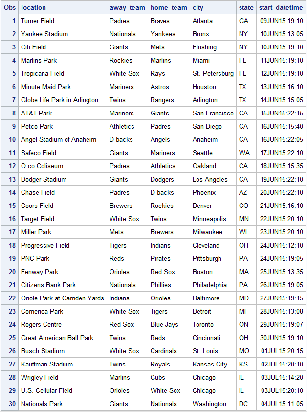
The traveling baseball fan problem is much harder than the TSP because it also incorporates scheduling constraints: a baseball fan must visit each of the 30 Major League ballparks exactly once, and each visit must include watching a scheduled Major League game. The objective is to minimize the time between the start of the first attended game and the end of the last attended game.

As the paper describes, some baseball fans really do this. For example, Chuck Booth worked out a 24-day schedule by hand for the 2009 season and actually attended the games, breaking a Guinness world record. In 2012, he broke his own record by completing a 23-day schedule. In both cases, Booth used a variety of modes of transportation, including airplanes, trains, rental cars, subways, and taxicabs. In 2008, Josh Robbins completed a 26-day schedule, traveling only by car.

Input Data

Major League Baseball has 30 teams, with stadiums throughout the United States plus one in Canada (Toronto). During the regular season (usually April through September), each team plays 162 games, for a total of $30 \cdot 162 / 2 = 2,430$ games. The input data that you need for the problem are date, starting time, location, and duration of each game, and travel times between stadiums. We got the game data from mlb.com by using a FILENAME statement with the URL access method. We got the travel times by using Google Maps, as demonstrated by Mike Zdeb in a 2010 SAS Global Forum paper.

Initial Formulation

One natural integer programming formulation involves a binary decision variable for each scheduled game, indicating whether the fan attends:
$\mathrm{Attend}[g]= \begin{cases} 1 & \text{if the baseball fan attends game $g$} \\ 0 & \text{otherwise} \end{cases}$

One set of constraints enforces the rule that the fan visits each stadium $s$ exactly once:
$\sum\limits_{\substack{g \in \text{GAMES}:\\ \mathrm{location}[g]= s}} \mathrm{Attend}[g]= 1$

Another set of constraints prevents the fan from attending any pair $(g_1,g_2)$ of games whose schedules conflict:
$\mathrm{Attend}[g_1] + \mathrm{Attend}[g_2] \le 1$

The corresponding PROC OPTMODEL code looks like this:

      /* Attend[g] = 1 if attend game g, 0 otherwise */
      var Attend {GAMES} binary;
 
      /* visit every stadium exactly once */
      con Visit_Once {s in STADIUMS}:
         sum {g in GAMES: location[g] = s} Attend[g] = 1;
 
      /* do not attend games that conflict */
      set CONFLICTS = {g1 in GAMES, g2 in GAMES: 
         location[g1] ne location[g2]
         and start_datetime[g1] <= start_datetime[g2] 
           < start_datetime[g1] + duration[g1] 
             + time_between_stadiums[location[g1],location[g2]]};
      con Conflict {<g1,g2> in CONFLICTS}:
         Attend[g1] + Attend[g2] <= 1;

Other variables and constraints are needed to encode the objective of minimizing total time, but for the sake of brevity I won't show them here---see the paper for details. It turns out that this formulation does not solve quickly, even with various improvements (some obtained by using the SOLVE WITH NETWORK statement introduced in SAS/OR 13.1) that are shown in the paper. After running the mixed integer linear programming (MILP) solver for one hour, there is still a large optimality gap.

Network Formulation

A reformulation as a side-constrained network flow problem yields much better solver performance. The network contains one node per game, plus a dummy source node and a dummy sink node to represent the start and end of the schedule, respectively, as shown using PROC SGPLOT here:

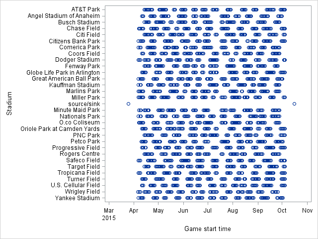
The (directed) arcs in the network are of three types:

• from the source node to each game node
• from each game node to the sink node
• from game $g_1$ to game $g_2$ if it is possible to attend game $g_1$ and then game $g_2$

The cost for each arc is the additional time incurred from the end of game $g_1$ to the end of game $g_2$. The goal is to find a shortest path that starts at the source, visits every stadium, and ends at the sink.

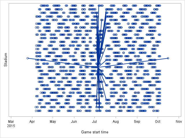
Without loss of optimality, for a given node you can instead consider only the shortest feasible arc to each stadium. Here is a plot of the arcs to and from an arbitrary game node in the network:

In the network formulation, the binary decision variables are associated with the arcs:
$\mathrm{UseArc}[g_1,g_2] = \begin{cases} 1 & \text{if the fan attends games $g_1$ and $g_2$ and no game in between} \\ 0 & \text{otherwise} \end{cases}$
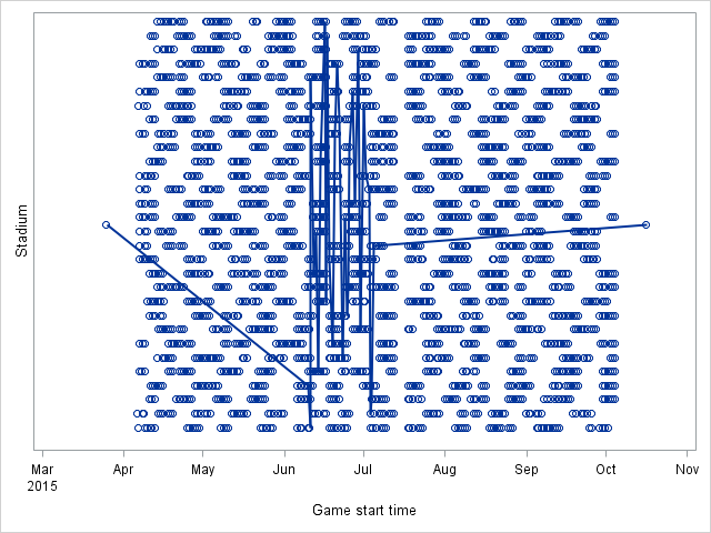
See the paper for the rest of the formulation. This network formulation has many more variables than the initial formulation but solves to optimality in less than an hour (and less than half an hour by using the parallel MILP solver). The resulting schedule completes the 30 games in 24.8 days of real time, or 26 calendar days.

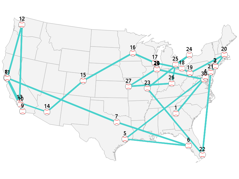
The resulting optimal path in the network looks like this:

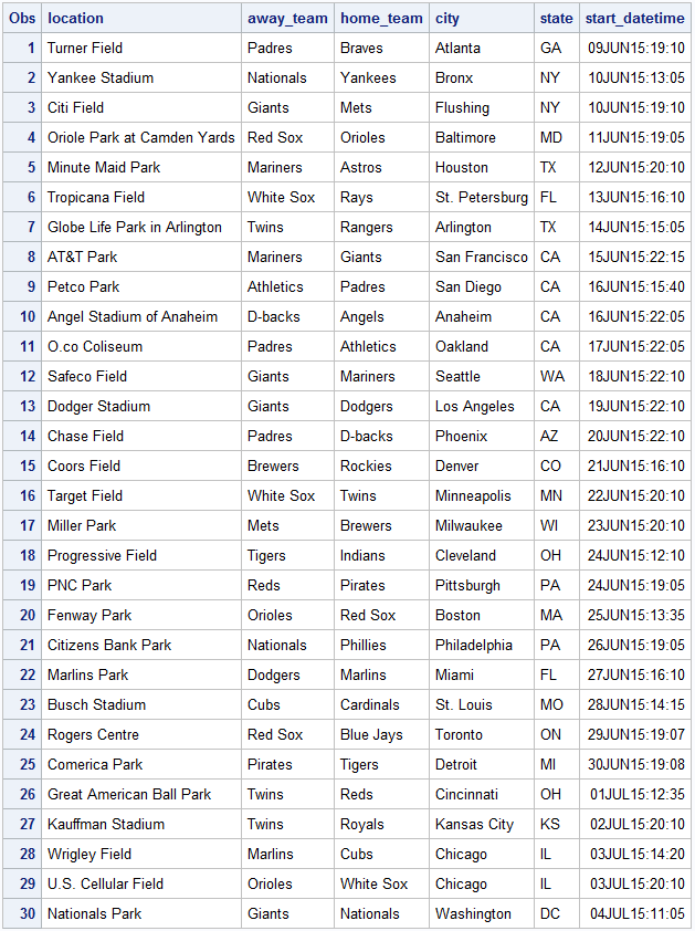
The resulting optimal schedule is as follows:

Geographically, the schedule looks like this (thanks to Robert Allison for the PROC GMAP code):

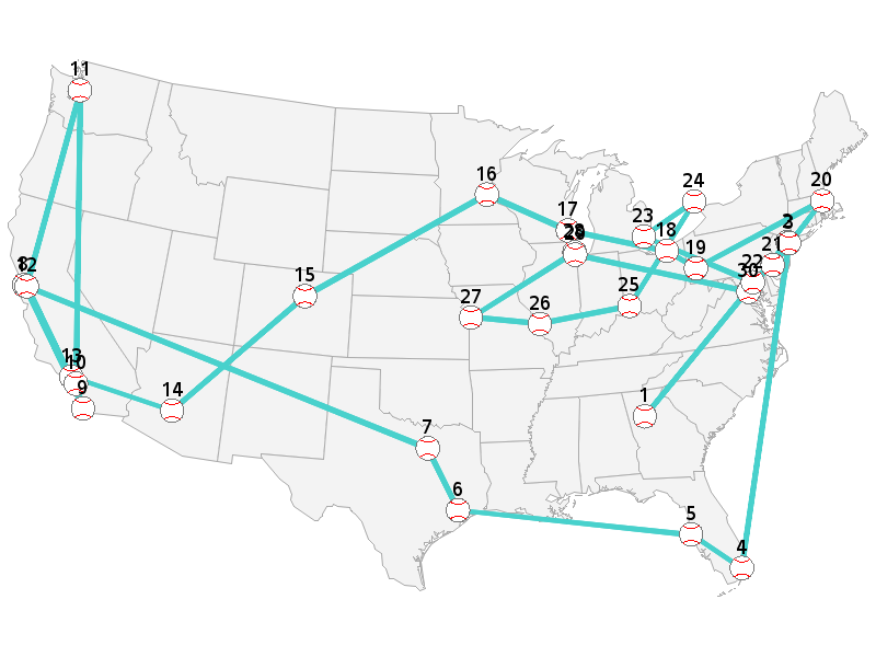
The paper also describes a secondary objective to minimize total distance traveled. The resulting optimal schedule starts and ends with the same two games as before but has some differences in the in-between games:

The new schedule reduces the distance traveled by about 3,100 miles (from about 18,850 miles to about 15,750 miles) and looks like this:

COFOR Statement

Besides the parallel MILP solver, another way to use parallel processing to solve the problem faster is to use the COFOR statement, which was introduced in SAS/OR 13.1. The COFOR statement operates in the same manner as the FOR statement, except that with the COFOR statement PROC OPTMODEL can execute the SOLVE statement concurrently with other statements.

Suppose that you know an upper bound $n$ on the number of days in an optimal schedule. Then you can divide and conquer the problem by considering each possible interval of $n$ consecutive days as a separate subproblem. Each of these subproblems (179, in both 2014 and 2015) has the same structure as the original problem but considers a much smaller subset of games, and an optimal solution to the original problem is among the optimal solutions to the subproblems.

You could use a FOR statement to loop through the start dates, fix the $\mathrm{UseArc}$ variables to 0 for arcs that include a game outside the current $n$-day subproblem, call the MILP solver, and unfix the variables that were fixed. But because the subproblems are independent of one another, you can solve them in parallel by simply changing the FOR statement to a COFOR statement instead, as in the following:

   cofor {d in START_DATES} do;
      put d=date9.;
      for {<g1,g2> in ARCS diff ARCS_d[d]} fix UseArc[g1,g2] = 0;
      solve;
      for {<g1,g2> in ARCS diff ARCS_d[d]} unfix UseArc[g1,g2];
      if substr(_solution_status_,1,7) = 'OPTIMAL' and bestObj > _OBJ_ then do;
         bestObj = _OBJ_;
         INCUMBENT = {<g1,g2> in ARCS: UseArc[g1,g2].sol > 0.5};
      end;
      put bestObj=;
   end;
   for {<g1,g2> in ARCS} UseArc[g1,g2] = (<g1,g2> in INCUMBENT);

The paper describes a slightly more sophisticated version that uses the MILP solver CUTOFF= option to terminate each subproblem early if the solver determines that the current subproblem cannot yield a better solution than the current best. It turns out that this entire COFOR loop finishes running in six minutes, yielding a provably optimal schedule. (Thanks to Leo Lopes for suggesting this use of COFOR. My first COFOR approach instead solved 2,430 problems, one per starting game, and took much longer.)

Extensions

See the paper for a discussion of various ways to extend the problem, such as:

• Use game-dependent game durations.
• Use time-dependent travel times.
• See each team exactly twice.
• See your favorite team at least $n$ times.
• See a particular matchup at least $n$ times.
• No repeat matchups.
• No consecutive games with the same team.
• Do not visit cold cities in April or September.
• Force a game to coincide with your existing travel plans to a city.
• Fix variables and reoptimize if your plan is disrupted (perhaps because of a game cancellation, extra innings, or traffic delays).

Applications

The traveling baseball fan problem is certainly interesting and a fun illustration of optimization, but I readily admit that it is useful to only a small segment of the population. However, you can imagine similar problems faced by a campaigning politician or a touring band, where a specified set of cities need to be visited but venues are available only on certain predetermined dates. The common generalization of these problems is called the traveling salesman problem with multiple time windows (TSPMTW). Even more generally, any optimization problem that involves routing and/or scheduling might benefit from the techniques described here and in the paper.