A customer asks if PROC TRANSREG can output the inflection points of a regression function. The answer is no, but you can easily find them by using PROC SGPLOT and some postprocessing. While you might never need to find inflection points, this post shows you how to run PROC SGPLOT, create smooth curves by using penalized B-splines, change the default threshold for disabling antialiasing, use ODS OUTPUT to create an output data set from PROC SGPLOT, process it, rename variables without necessarily knowing the precise original names, create an additional data set to plot, merge the two data sets, create a plot from the merged data, and display drop lines and reference lines using the values of variables. This theme of using ODS OUTPUT along with PROC SGPLOT is going to carry over into my next two posts as well.

If your math skills are a bit rusty, an inflection point is a point on a curve at which the sign of the curvature changes (http://mathworld.wolfram.com/InflectionPoint.html). Don't worry if that does not seem relevant to you. Code that does all the math is provided, and the graphical lessons from this post do not depend on understanding the math. The following graph shows two functions and their three inflection points.

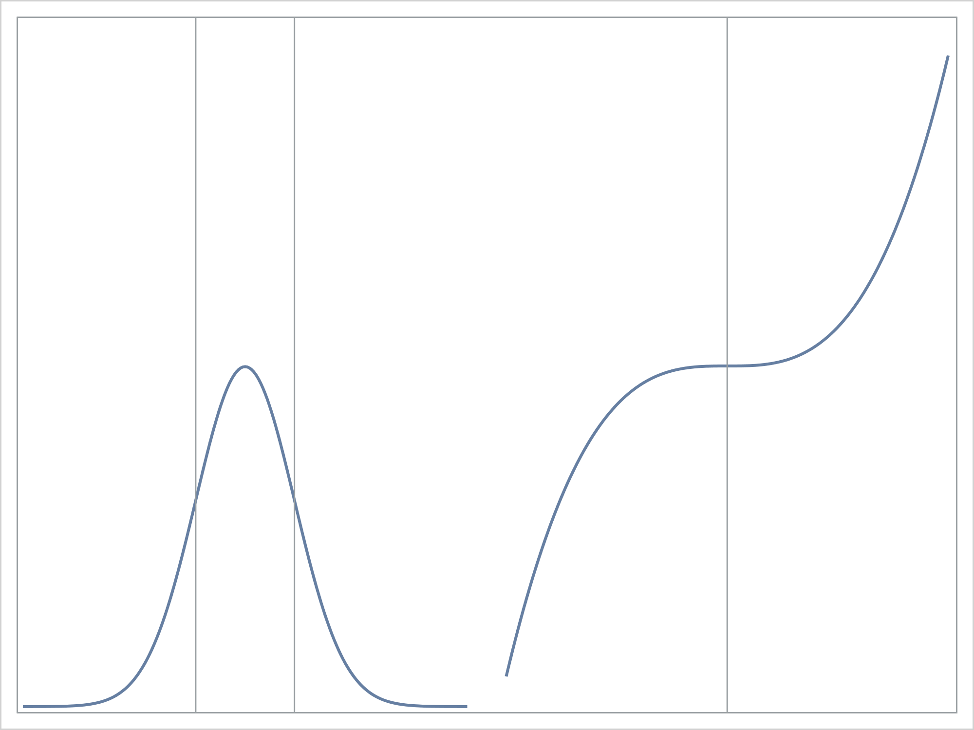
The following statement sets the antialiasing maximum to 10,000. When antialiasing is in effect, lines, curves, and other features of the graph are rendered in a cleaner way. Antialiasing is computationally expensive, so it is disabled in some graphs. Subsequent options such as the PBSPLINE option MAXPOINTS=5000 create 4,999 line segments. This along with other graph features disable antialiasing at the default value of ANTIALIASMAX=4000.

ods graphics on / antialiasmax=10000;

The data and the preceding graph are created by the following two steps.

data x(drop=c);
   c = 1 / sqrt(2 * constant('pi'));
   do x = -4.5 to 4.5 by 0.05;
      y1 = c * exp(-0.5 * x * x);
      y2 = x ** 3;
      output;
   end;
run;
 
proc sgplot noautolegend nocycleattrs;
   ods output sgplot=sg;
   pbspline y=y1 x=x / nomarkers;
   refline -1 1 / axis=x;
   pbspline y=y2 x=x / nomarkers y2axis x2axis;
   refline 0 / axis=x2;
   xaxis display=none offsetmax=0.52;
   yaxis display=none offsetmax=0.5;
   x2axis display=none offsetmin=0.52;
   y2axis display=none;
run;

The PBSPLINE statement fits penalized B-splines, which display a curve in a scatter plot. You can use two X and two Y axes and offsets when you want to display two graphs side-by-side. Here, since we have a series of points on each of two curves, we could have used a SERIES plot instead. We will need PBSPLINE later on when we fit a function to data and find the inflection points. First, let's stick with a function. The following steps create and display a standard normal density function.

data x(drop=c);
   c = 1 / sqrt(2 * constant('pi'));
   do x = -4.5 to 4.5 by 0.05;
      y = c * exp(-0.5 * x * x);
      output;
   end;
run;
 
proc sgplot noautolegend data=x;
   ods output sgplot=sg;
   pbspline y=y x=x / nomarkers maxpoints=5000;
   xaxis display=(nolabel);
   yaxis display=(nolabel);
run;

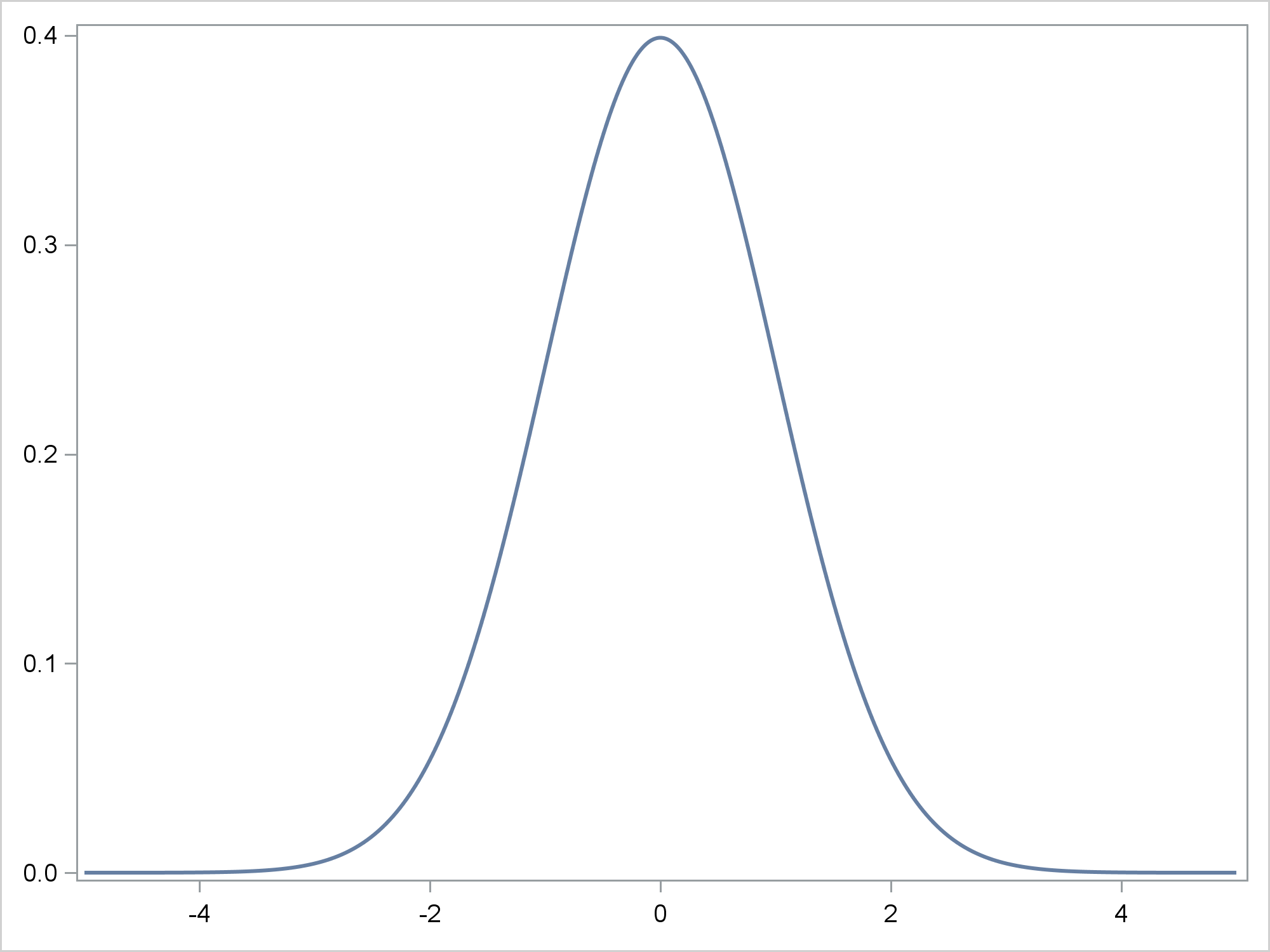
The MAXPOINTS= option in the PBSPLINE statement controls the number of points for which X and Y coordinates for the penalized B-spline function are computed. Five-thousand points is considerably more than the original number of data points. This enables a more precise evaluation of the location of the inflection points. The ODS OUTPUT statement creates a SAS data set from the data object that is used to make the graph.

You might not think of using PROC SGPLOT and ODS OUTPUT to create results for future processing. In this case, it is quite handy. The original question I received pertained to PROC TRANSREG. Both PROC TRANSREG and PROC SGPLOT call the same code to fit penalized B-splines. The difference is that PROC TRANSREG does not automatically create points that are needed to evaluate the function at regular intervals. PROC TRANSREG only evaluates the penalized B-spline function at actual data points. If you want a smoother function, you have to make a list of points in a DATA step, append them to the data, and feed them in as passive observations (for example by giving them zero frequencies). This is all easier in PROC SGPLOT, because the PBSPLINE statement has a MAXPOINTS= option. It is not much of an issue when the data set contains coordinates for a mathematical function such as in this example. It becomes an issue with real or artificial data where the X values are not uniformly generated.

The ODS OUTPUT data set might be similar to the input data set, or it might be quite different. Let's look at the variable names. This is the way I normally run PROC CONTENTS when I only want to see the variable names.

proc contents varnum; ods select Position; run;

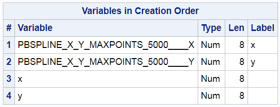
PROC SGPLOT manufactures two names. They contain the X and Y coordinates for the penalized B-spline function. The names are long and hard to type. Furthermore if you change the MAXPOINTS= option, the names change. Since you might want to change the number of points, it is convenient to have a mechanism to rename these variables no matter what their original names are. The following steps create a macro variable &Ren that changes the two long names to PBX and PBY.

proc contents noprint data=sg out=names; run;
 
data _null_;
   set names(obs=2);
   length ren $ 100;
   retain ren ' ';
   ren = catx(' ', ren, name, '=',
              cats(substr(name, 1, 2), substrn(name, length(name), 1)));
   call symputx('ren', ren);
run;

They do this by processing the PROC CONTENTS output data set of names to generate RENAME= data set option syntax.

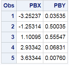
The following step finds the inflection points and outputs them to a data set.

data inf(keep=pbx pby);
   set sg(drop=x y rename=(&ren));
   der2 = (lag2(pby) - 2*lag(pby) + pby) / (pbx - lag(pbx)) ** 2;
   if n(lag(der2)) and (sign(lag(der2)) ne sign(der2)) then output;
run;

It reads the output data set that ODS made from the data object that underlies the graph. It renames the variables. It computes the second derivative of the penalized B-spline function. This DATA step uses LAG functions, which begin by initializing their queues to missing. Hence this DATA step produces notes about performing operations on missing values. In many cases, this note is a cause for concern. In this case, it is not. The DATA step outputs the X and Y values when the sign of the second derivative changes. Since these are numerical derivatives derived from a finite number of points, we will not get exactly the right results, but they should be close. For a regression function the results will certainly be close enough. This step displays the inflection points.

proc print; run;

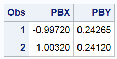
These values are close to the true X values of -1 and 1.

The following step merges the two data sets

data all;
   merge x inf;
run;

The merged data set contains the two variables from the original data set, X and Y. These variables have 181 nonmissing observations. It also contains two additional variables that contain the inflection points, PBX and PBY. These variables have 2 nonmissing observations and 179 missing observations. Large blocks of missing values can be perfectly normal when you are creating graphs by overlying different plot types.

The following step displays the normal density function and the inflection points.

proc sgplot noautolegend;
   title 'Inflection Points';
   pbspline y=y x=x / nomarkers;
   dropline x=pbx y=pby;
   xaxis display=(nolabel);
   yaxis display=(nolabel);
run;
title;

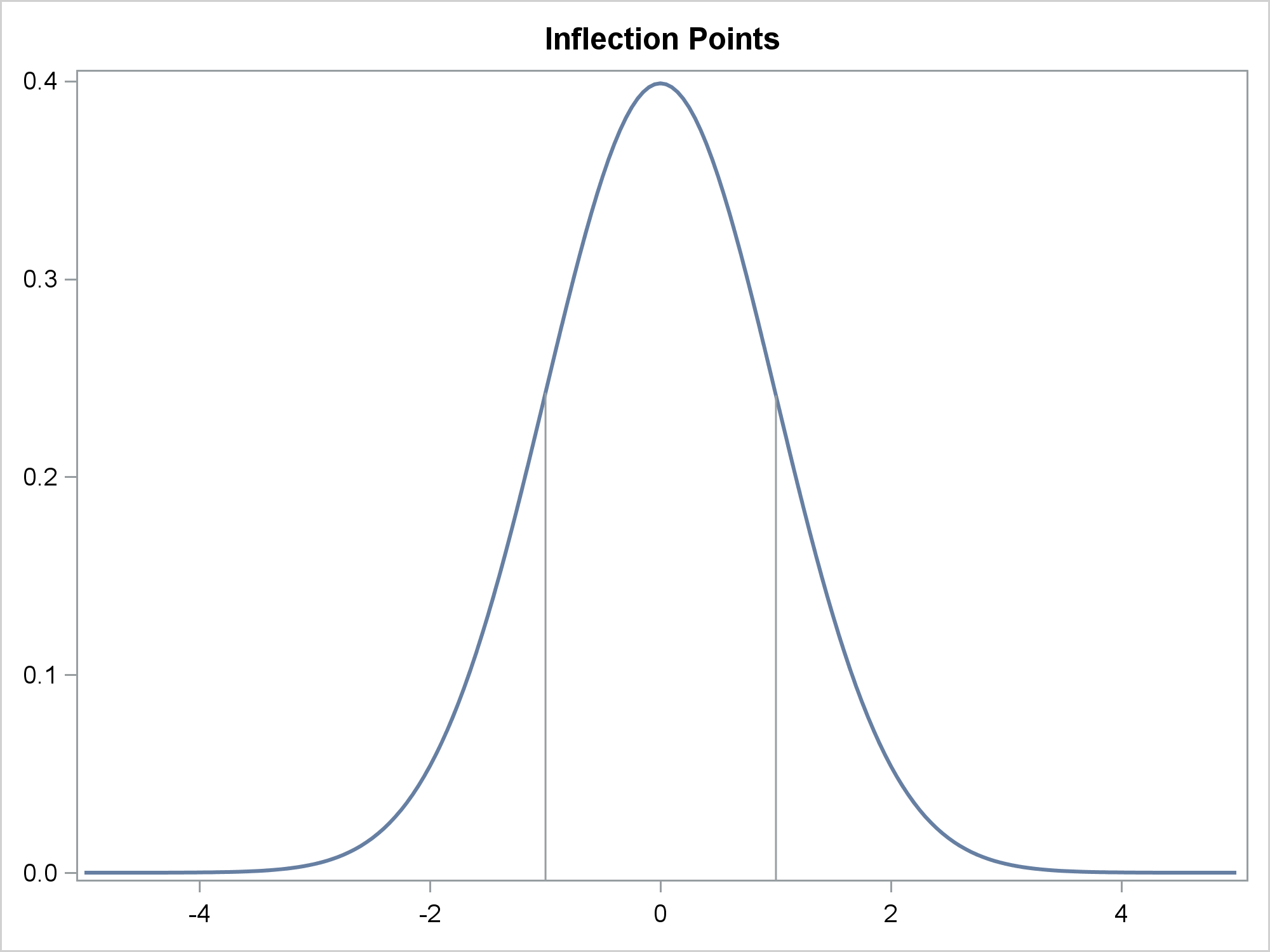
You specify the PBX and PBY variables in the DROPLINE statement.

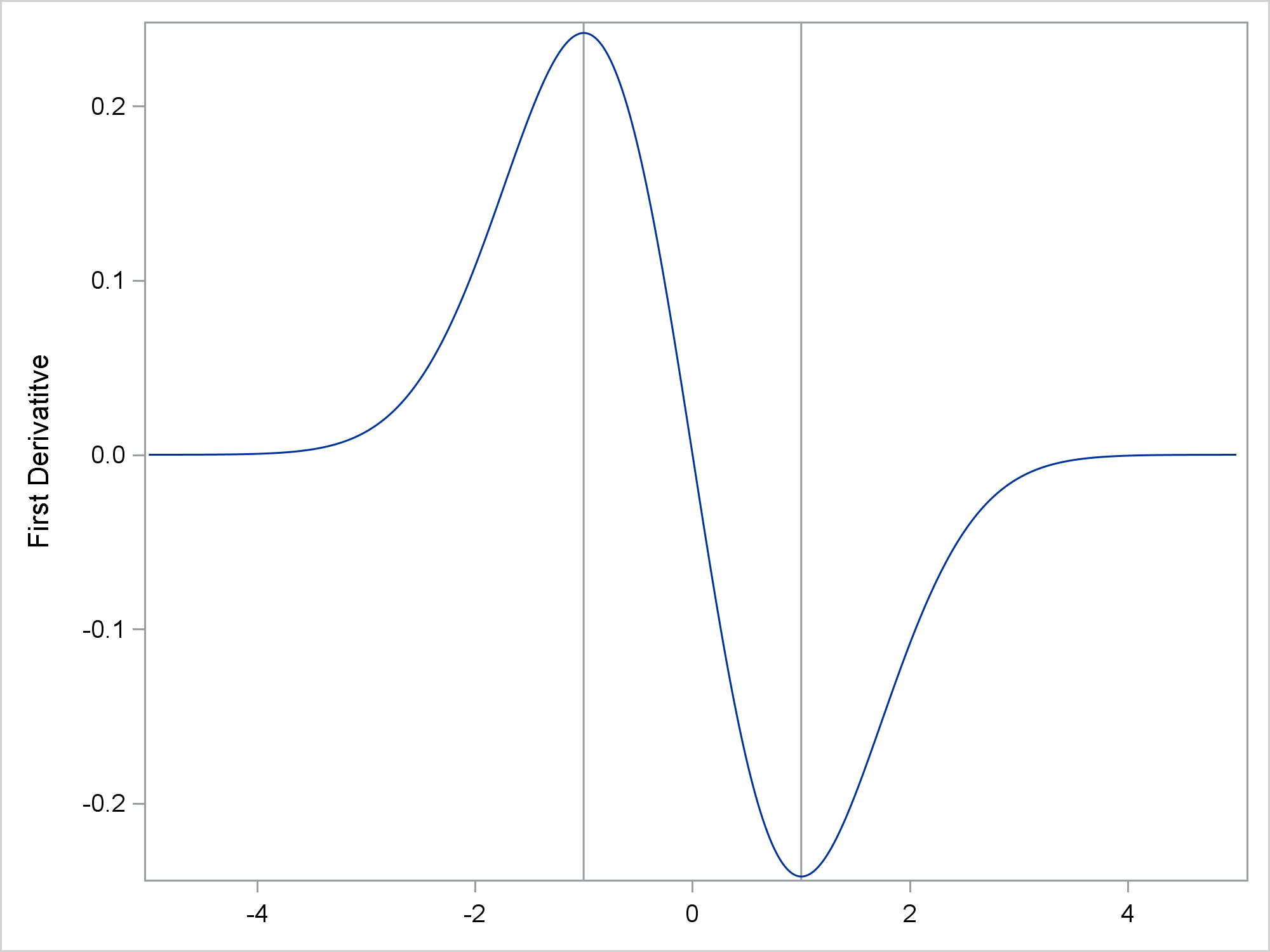
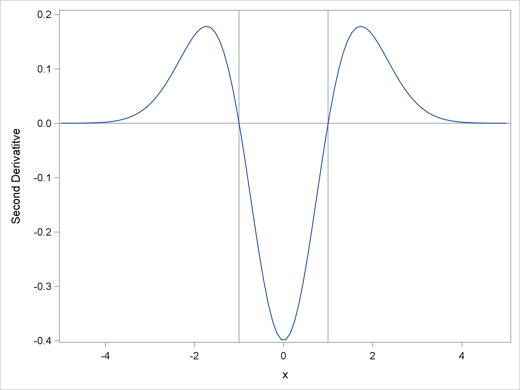
The following steps store the first and second derivatives in a data set and plot them.

data ders;
   set sg(rename=(&ren));
   der1 = (pby - lag(pby)) / (pbx - lag(pbx));
   der2 = (lag2(pby) - 2*lag(pby) + pby) / (pbx - lag(pbx)) ** 2;
run;
 
proc sgplot noautolegend;
   refline -1 1 / axis=x;
   series y=der1 x=pbx;
   xaxis display=(nolabel);
   yaxis label='First Derivatitve';
run;
 
proc sgplot noautolegend;
   refline -1 1 / axis=x;
   refline 0 / axis=y;
   series y=der2 x=pbx;
   yaxis label='Second Derivatitve';
run;

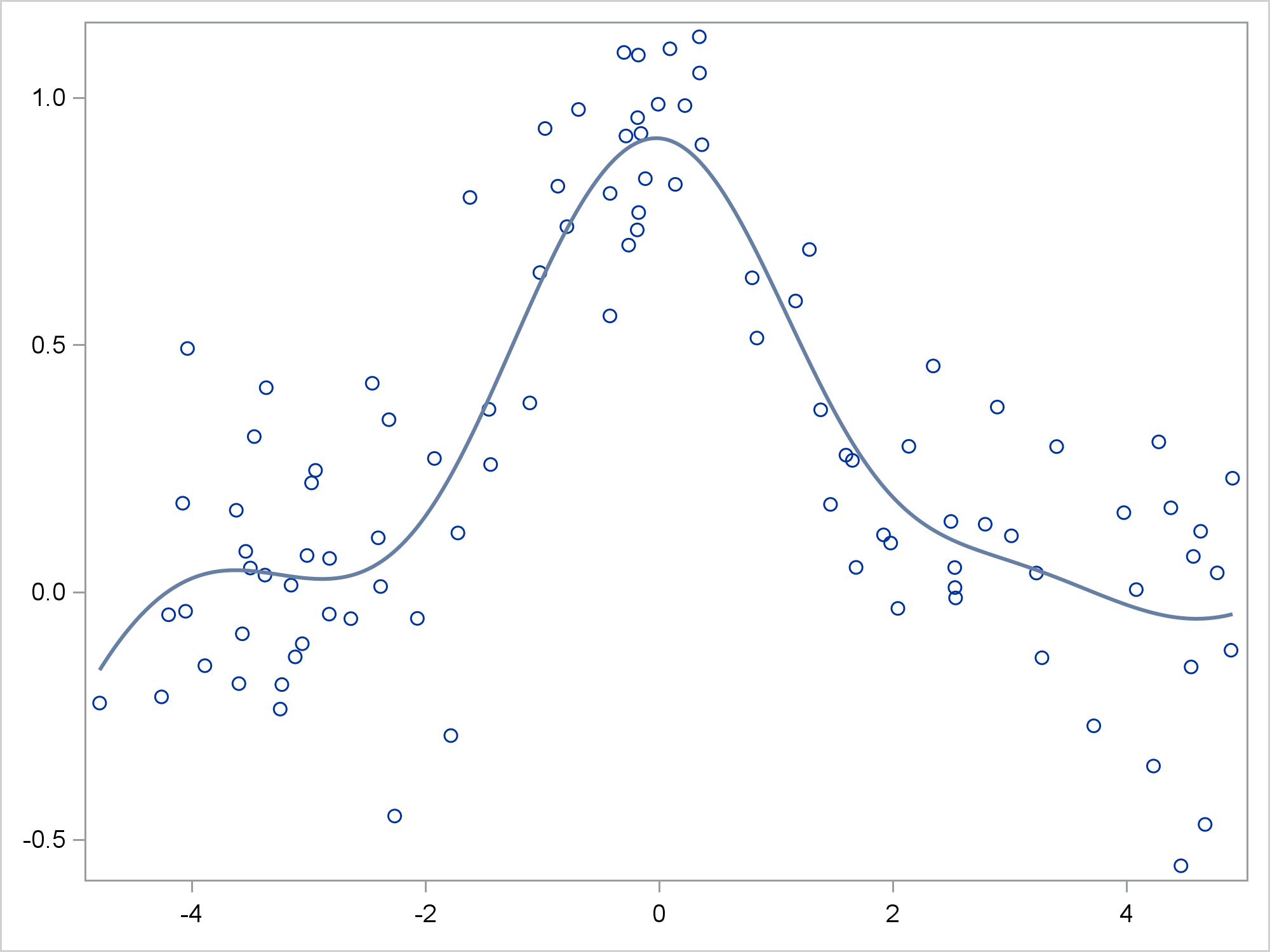
Now, back to the original question that I was asked. Next, I will make some random data that have normal error, so a regression function needs to be found.

data x2(drop=i);
   do i = 1 to 100;
      x = 10 * uniform(104) - 5;
      y = exp(-0.5 * x * x) + 0.2 * normal(104);
      output;
   end;
run;

The following step displays the penalized B-spline fit function and outputs it to an ODS OUTPUT data set.

proc sgplot noautolegend data=x2;
   ods output sgplot=sg;
   pbspline y=y x=x / maxpoints=5000;
   xaxis display=(nolabel);
   yaxis display=(nolabel);
run;

The following steps rename the manufactured variables.

proc contents noprint data=sg out=names; run;
 
data _null_;
   set names(obs=2);
   length ren $ 100;
   retain ren ' ';
   ren = catx(' ', ren, name, '=',
              cats(substr(name, 1, 2), substrn(name, length(name), 1)));
   call symputx('ren', ren);
run;

The next steps find and display the inflection points.

data inf(keep=pbx pby);
   set sg(drop=x y rename=(&ren));
   der2 = (lag2(pby) - 2*lag(pby) + pby) / (pbx - lag(pbx)) ** 2;
   if n(lag(der2)) and (sign(lag(der2)) ne sign(der2)) then output;
run;
 
proc print; run;

The next steps merge the two data sets and display the inflection points.

data all2;
   merge x2 inf;
run;
 
proc sgplot noautolegend;
   title 'Inflection Points';
   pbspline y=y x=x;
   dropline x=pbx y=pby;
   xaxis display=(nolabel);
   yaxis display=(nolabel);
run;
title;

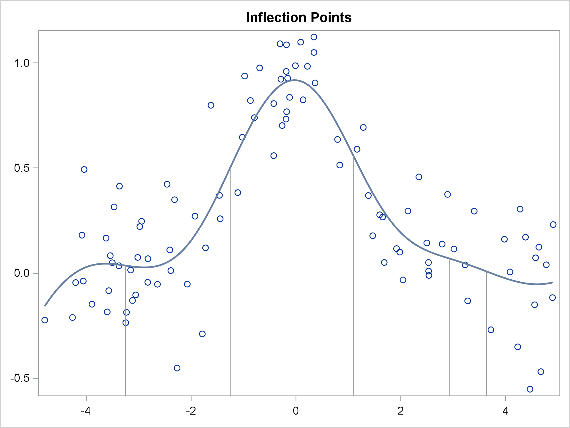
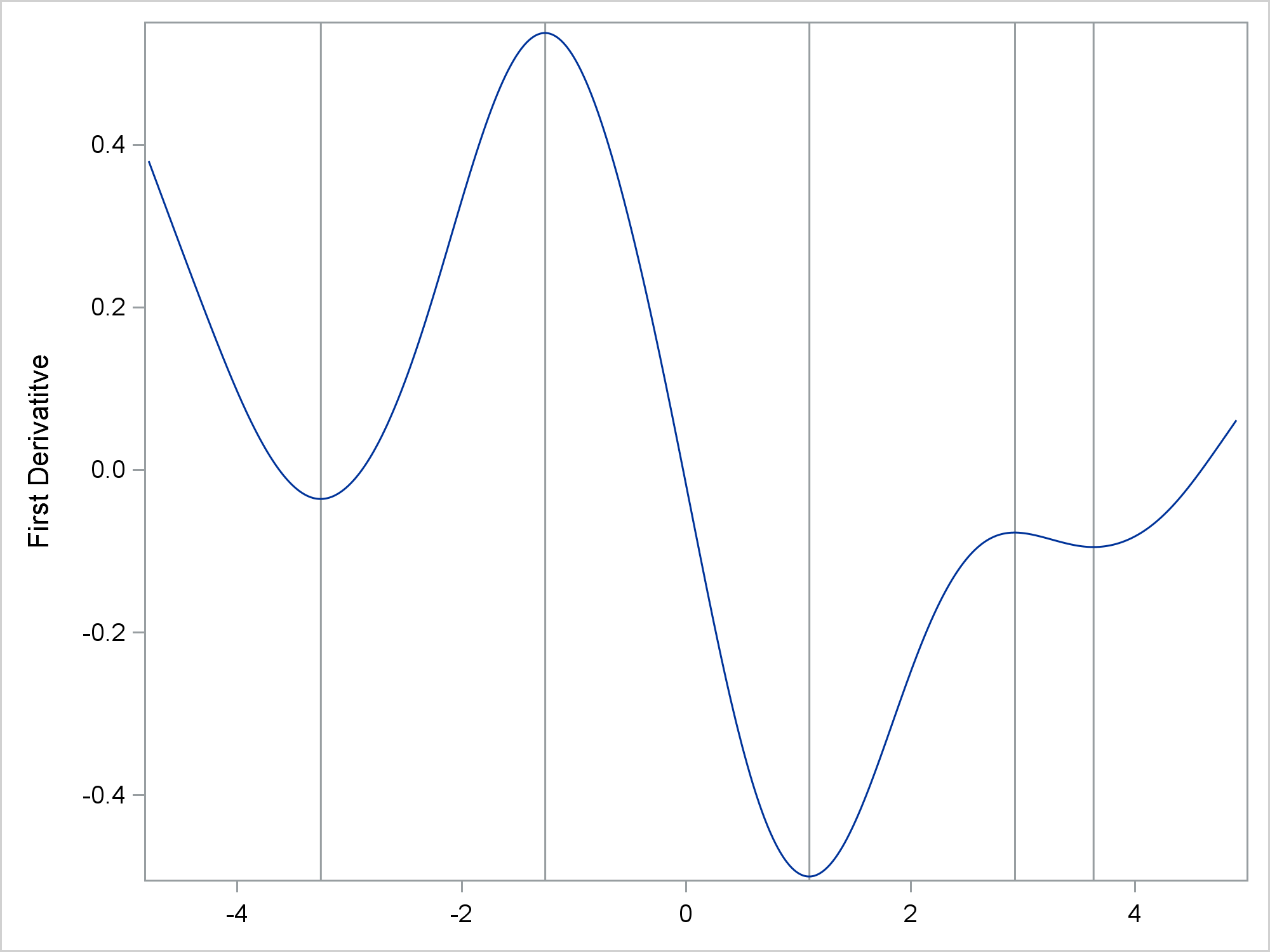
Since the fit function changes directions several times, there are multiple inflection points. The following steps compute the first derivative of the fit function and display it along with the inflection points.

data ders;
   set sg(rename=(&ren));
   der1 = (pby - lag(pby)) / (pbx - lag(pbx));
run;
 
data ders;
   merge ders inf(keep=pbx rename=(pbx=ix));
run;
 
proc sgplot noautolegend;
   refline ix / axis=x;
   series y=der1 x=pbx;
   xaxis display=(nolabel);
   yaxis label='First Derivatitve';
run;

I'm pleased that you read this far! Even if you don't understand all of the calculus, I hope you can see the beauty in these plots. Thanks to my colleague Rick Wicklin from the DO Loop Blog for helping me with the direct method of computing the second numerical derivative.