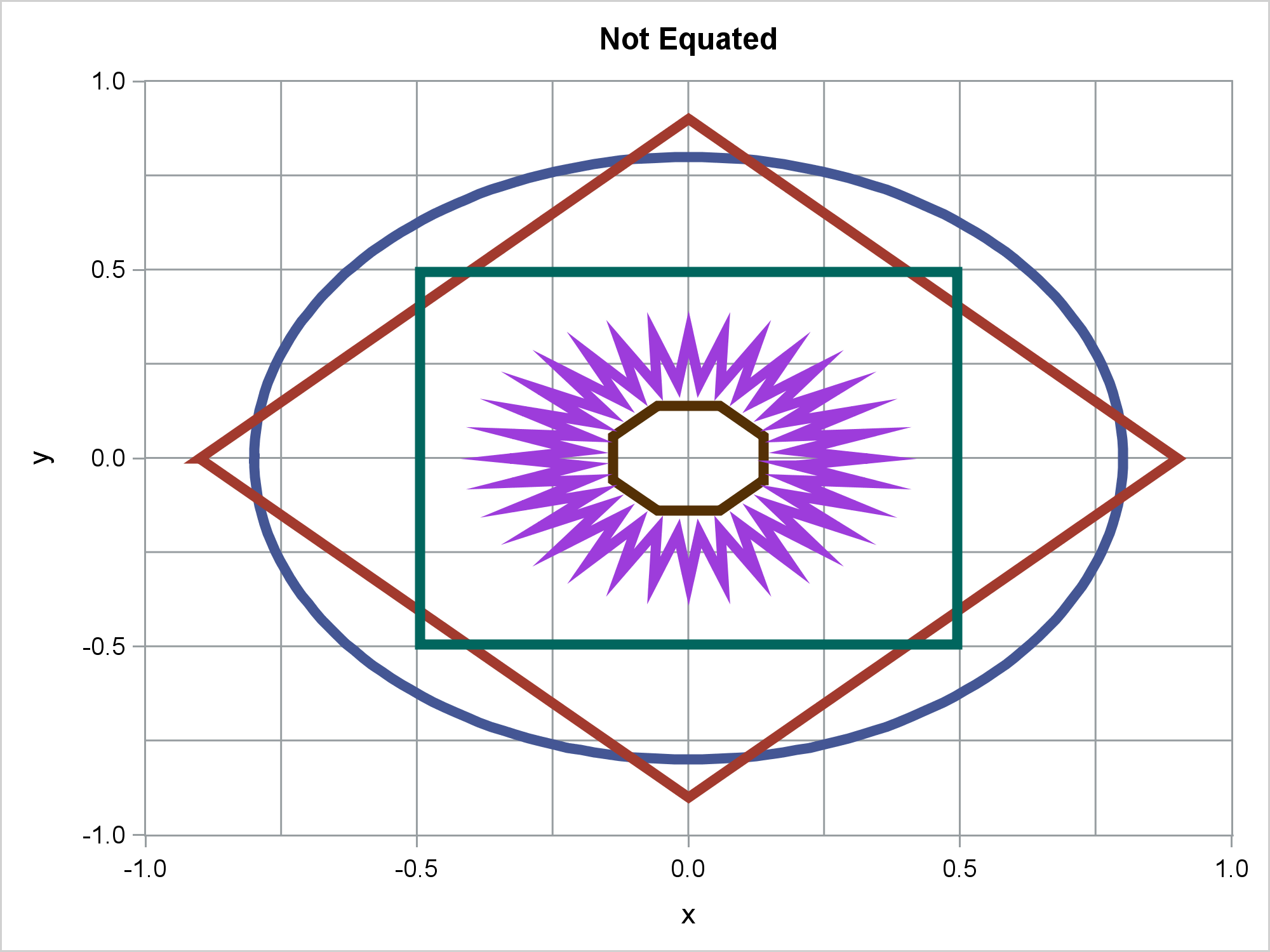
Creating a graph that has equated axes is a subject that has been near and dear to my heart since I was in graduate school. Axes are equated when a centimeter on one axis represents the same data range as a centimeter on the other axis. Equated axes are important when displaying geometric shapes and results from analyses such as principal component analysis. Equated axes respect and portray the geometry of the analysis.

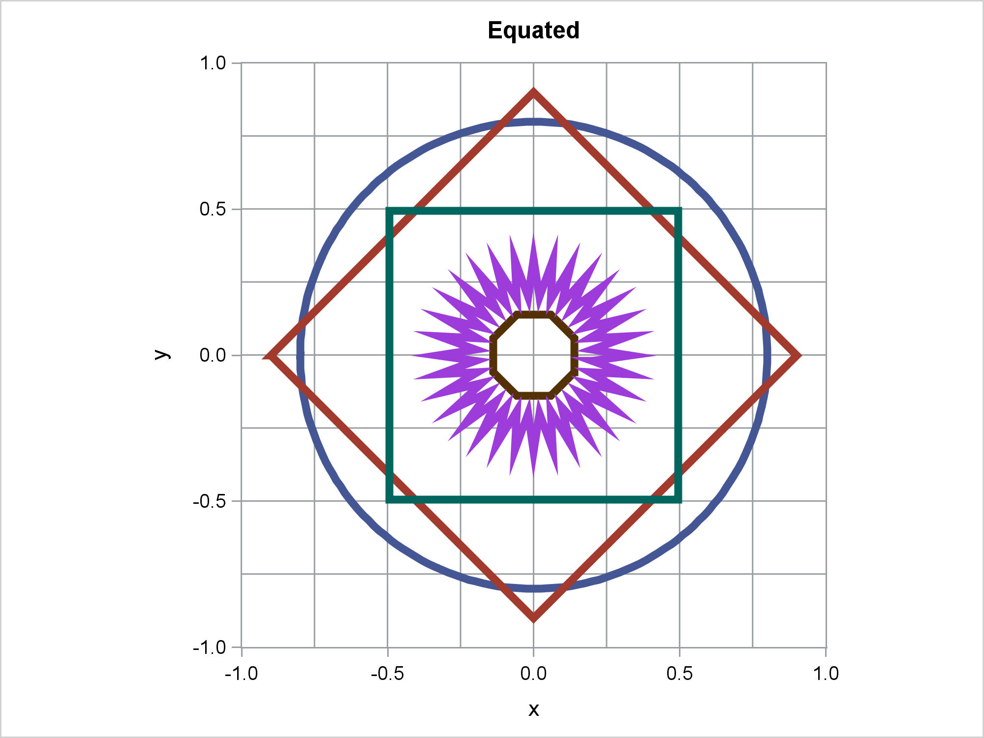
Click to enlarge.

It hasn't always been easy to equate axes in SAS. Decades ago, when I was a fairly new SAS/STAT developer, I successfully lobbied for options in PROC PLOT to make it easier to equate axes. Later, when I wrote the %PlotIt macro (which makes entire plots using PROC GANNO), I made equated axes a central part of it. I also wrote an %Equate macro for use with PROC GPLOT. We have come a long ways since then! Now the GTL has extensive options for equated axes, and PROC SGPLOT has options as well. This post shows you some of those options (in particular the ASPECT= option) and provides examples of what they do.

Most graphs do not use equated axes and for good reason. For most graphs, it does not make sense to equate axes. If you have a scatter plot of height and weight, family size and income, age and blood pressure, or any of an unlimited number of pairs of variables that are on different scales, then you would not want to try to equate axes. You want what ODS Graphics automatically does--it fills the available space in the graph. However, equated axes are important for principal component analysis, correspondence analysis, multidimensional scaling, and other analyses. Equated axes are also important when displaying geometric shapes such as squares and circles. Unless you equate the axes, you will display rectangles instead of squares and ovals instead of circles. Bubble plots and maps would look pretty silly if they did not pay attention to the proper geometry.

Sanjay has several nice examples of graphs that use circles. For examples, see Polar Graph and Polar Graph - Wind Rose. Sanjay uses PROC SGPLOT and the option ASPECT=1 to create graphs with circles. The aspect ratio is the ratio of the height divided by the width. When the aspect ratio is one, the graph is square. It is easy to equate axes for a circle since a circle fits in a square (that is, the ranges of coordinates for both the X and Y axes are the same). When the aspect ratio is less than one, the graph is wider than it is tall. When the aspect ratio is greater than one, the graph is taller than it is wide. I discuss ASPECT=1, but I also discuss methods that work when the graph area is not square. I mention LAYOUT OVERLAYEQUATED in the GTL, but I mostly discuss PROC SGPLOT and a more heuristic approach to equating axes.

This first DATA step creates coordinates for 200 points that fall on a circle. (There are 201 observations because the first and last observations both contain the same point.)

data x(drop=pi tau);
   pi = constant('pi');
   do tau = -pi to pi by pi / 100;
      x = cos(tau);
      y = sin(tau);
      output;
   end;
run;

The following step displays these points.

proc sgplot data=x;
   series y=y x=x;
run;

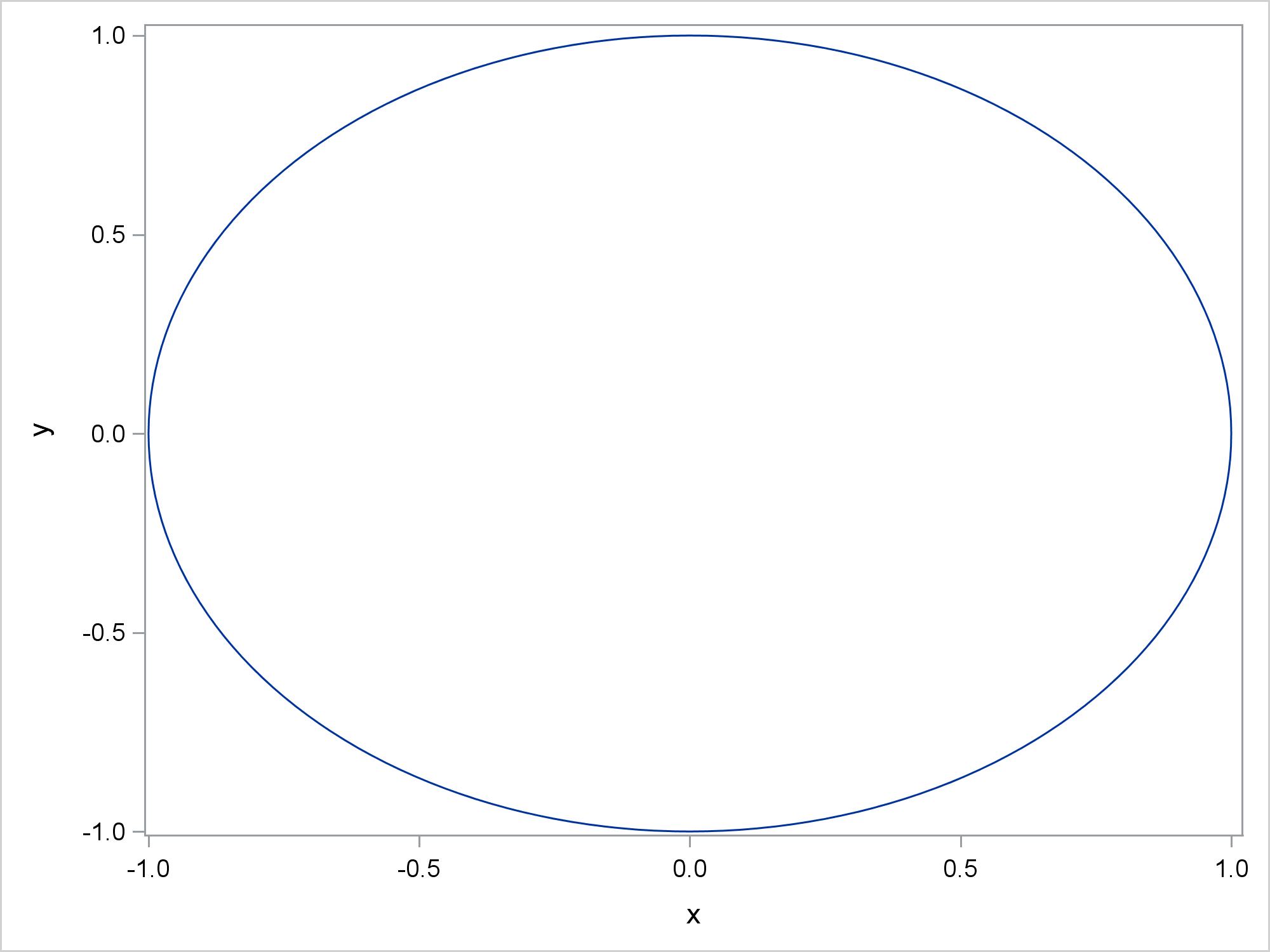
Because the axes are not equated, the graph displays an oval. The next step specifies the option ASPECT=1 and displays a circle.

%let o offsetmin=0.02 offsetmax=0.02;
proc sgplot data=x aspect=1;
   series y=y x=x;
   xaxis &o;
   yaxis &o;
run;

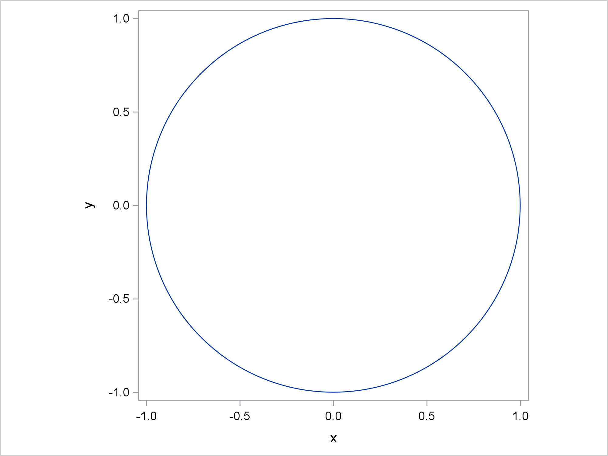
Offsets (or padding at the end of each axis) can vary slightly across the minimum and maximum of both axes. Specifying consistent offsets along with ASPECT=1 and equal X and Y axis ranges ensures that the axes are equated.

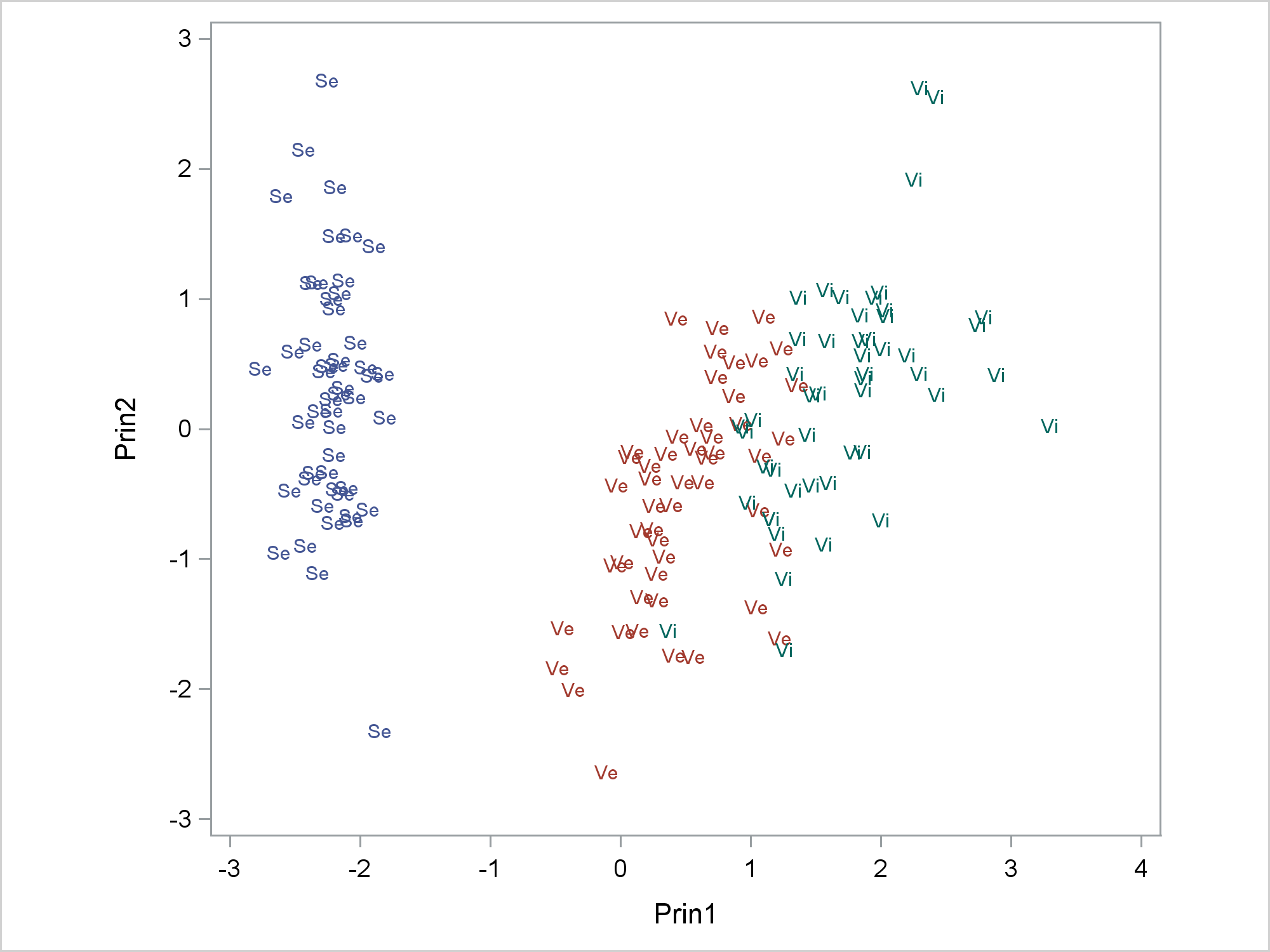
PROC PRINCOMP displays plots that have equated axes. This step displays scores on the first two principal components.

ods graphics on;
proc princomp data=sashelp.iris out=scores plots=score;
  ods select '2 by 1';
run;

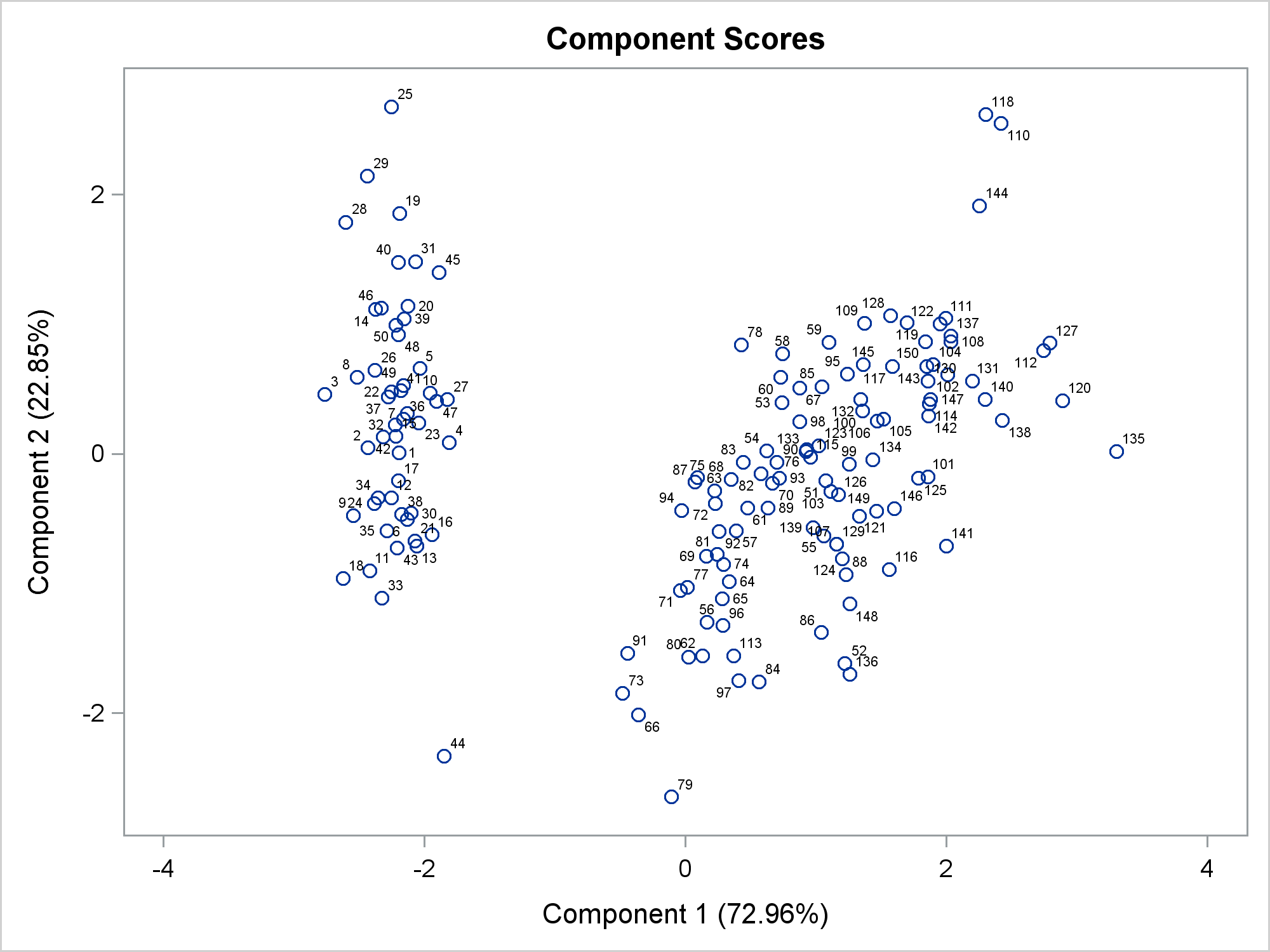
Both axes have the same tick increment (which is not required). Most importantly, the same data range is displayed on each axis by using the same distance. You can display the graph template by submitting the following step.

proc template; 
  source Stat.Princomp.Graphics.ScorePlot;
quit;

I will not show you the template. I just want to point out that this statement equates the axes:

layout overlayequated / equatetype=fit ...;

Procedures such as PRINCOMP, PRINQUAL, CORRESP, TRANSREG, MDS, and many others automatically use LAYOUT OVERLAYEQUATED to equate axes in some graphs.

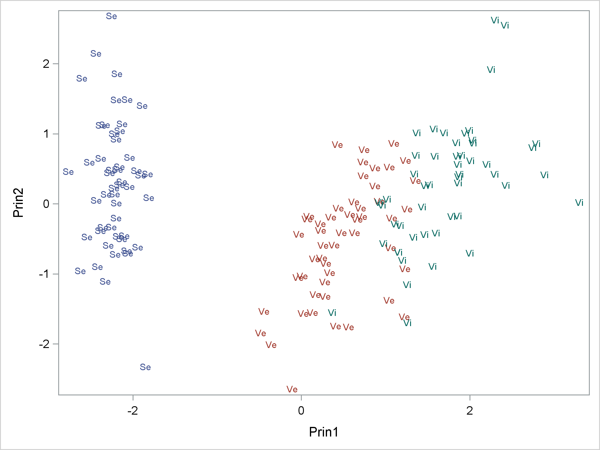
You can also display the principal component scores by using PROC SGPLOT and the output data set from PROC PRINCOMP, but the axes are not equated.

proc sgplot noautolegend;
   scatter y=prin2 x=prin1 / markerchar=species group=species;
   format species $2.;
run;

You can specify ASPECT=1, which makes the plot square, but the axes are still not equated because the X and Y axis variables have different ranges.

proc sgplot noautolegend aspect=1;
   scatter y=prin2 x=prin1 / markerchar=species group=species;
   format species $2.;
run;

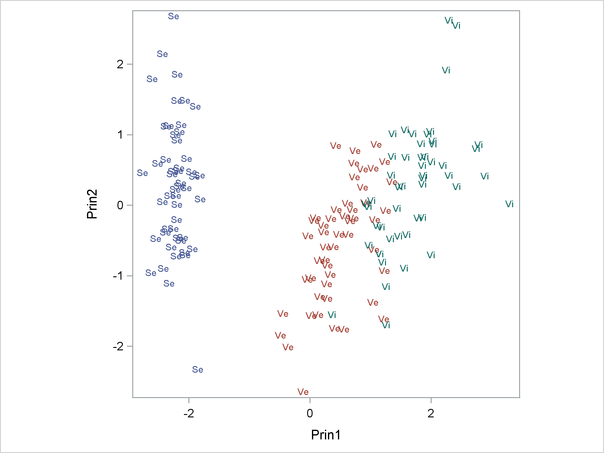
Specifying an aspect ratio controls the relative length of the axes, but it does not always equate them. Specifying an aspect ratio of one will only equate the axes when the ranges of coordinates are the same for both the X and Y axes.

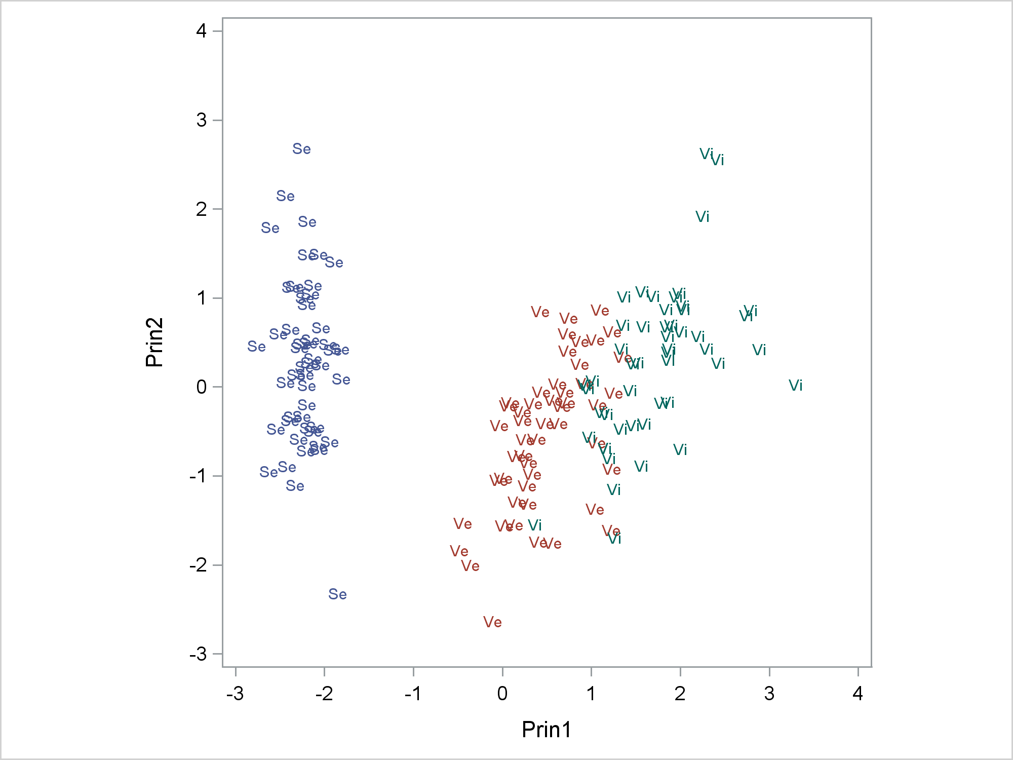
The next two steps create a square plot that has equated axes. Notice that the &o (options) macro variable specifies consistent offsets for both ends of both axes.

data _null_;
   set scores end=eof;
   retain min max;
   if _n_ = 1 then do; min = prin1; max=prin1; end;
   min = min(min, prin1, prin2);
   max = max(max, prin1, prin2);
   if eof then do;
      range = max - min;
      inc = 10 ** ceil(log10(range) - 1.0);
      if range / inc >= 7.5 then inc = inc * 2;
      if range / inc <= 2.5 then inc = inc / 2;
      if range / inc <= 2.5 then inc = inc / 2;
      call symputx('min', floor(min / inc) * inc);
      call symputx('max', ceil (max / inc) * inc);
      call symputx('inc', inc);
   end;
run;
 
%put &min &max &inc;
 
proc sgplot noautolegend aspect=1;
   scatter y=prin2 x=prin1 / markerchar=species group=species;
   format species $2.;
   xaxis values=(&min to &max by &inc) &o;
   yaxis values=(&min to &max by &inc) &o;
run;

The DATA step processes the X and Y variables, finds the minimum of the two minima, the maximum of the two maxima, and uses them to find a common set of ticks for both axes. Now ASPECT=1 produces a plot that shows the proper geometry. The IF block finds the range of values (across both variables), and initializes the increment to a power of ten. Then it tests the initial increment. If there are too many ticks, a larger increment is used. If there are too few ticks, a smaller increment is used. If there are still too few ticks, an even smaller increment is used. Next, the minimum and maximum are set to multiples of the increment. These values are output to macro variables for use in PROC SGPLOT.

You can incorporate that code into a macro as follows.

%macro equate(x, y, data=_last_, type=square);
data _null_;
   set &data end=eof;
   retain _minx _maxx _miny _maxy;
   if _n_ = 1 then do; _minx = &x; _maxx=&x; _miny = &y; _maxy=&y; end;
   _minx = min(_minx, &x);
   _maxx = max(_maxx, &x);
   _miny = min(_miny, &y);
   _maxy = max(_maxy, &y);
   if eof and lowcase("&type") eq 'square' then do;
      range = max(_maxy, _maxx) - min(_miny, _minx);
      inc = 10 ** ceil(log10(range) - 1.0);
      if range / inc >= 7.5 then inc = inc * 2;
      if range / inc <= 2.5 then inc = inc / 2;
      if range / inc <= 2.5 then inc = inc / 2;
      call symputx('minx', floor(min(_miny, _minx) / inc) * inc, 'G');
      call symputx('maxx',  ceil(max(_maxy, _maxx) / inc) * inc, 'G');
      call symputx('miny', floor(min(_miny, _minx) / inc) * inc, 'G');
      call symputx('maxy',  ceil(max(_maxy, _maxx) / inc) * inc, 'G');
      call symputx('inc', inc, 'G');
      call symputx('aspect', 1, 'G');
   end;
   else if eof then do;
      rangex = _maxx - _minx;
      rangey = _maxy - _miny;
      range  = max(rangex, rangey);
      inc = 10 ** ceil(log10(range) - 1.0);
      if range / inc >= 7.5 then inc = inc * 2;
      if range / inc <= 2.5 then inc = inc / 2;
      if range / inc <= 2.5 then inc = inc / 2;
      minx = floor(_minx / inc) * inc;
      maxx = ceil (_maxx / inc) * inc;
      miny = floor(_miny / inc) * inc;
      maxy = ceil (_maxy / inc) * inc;
      call symputx('minx', minx, 'G');
      call symputx('maxx', maxx, 'G');
      call symputx('miny', miny, 'G');
      call symputx('maxy', maxy, 'G');
      call symputx('inc', inc, 'G');
      call symputx('aspect', (maxy - miny) / (maxx - minx), 'G');
   end;
run;
%mend;

The following steps create the same results that were shown in the preceding graph.

%equate(prin1, prin2, data=scores)
 
%put &minx &maxx &miny &maxy &inc &aspect;
 
proc sgplot data=scores noautolegend aspect=&aspect;
   scatter y=prin2 x=prin1 / markerchar=species group=species;
   format species $2.;
   xaxis values=(&minx to &maxx by &inc) &o;
   yaxis values=(&miny to &maxy by &inc) &o;
run;

The next step uses the option TYPE=RECTANGLE. This option still picks a common tick increment, but it enables different minima and maxima. The aspect ratio (approximately 0.86) along with the carefully chosen minima and maxima create equated axes.

%equate(prin1, prin2, data=scores, type=rectangle)
 
%put &minx &maxx &miny &maxy &inc &aspect;
 
proc sgplot data=scores noautolegend aspect=&aspect;
   scatter y=prin2 x=prin1 / markerchar=species group=species;
   format species $2.;
   xaxis values=(&minx to &maxx by &inc) &o;
   yaxis values=(&miny to &maxy by &inc) &o;
run;

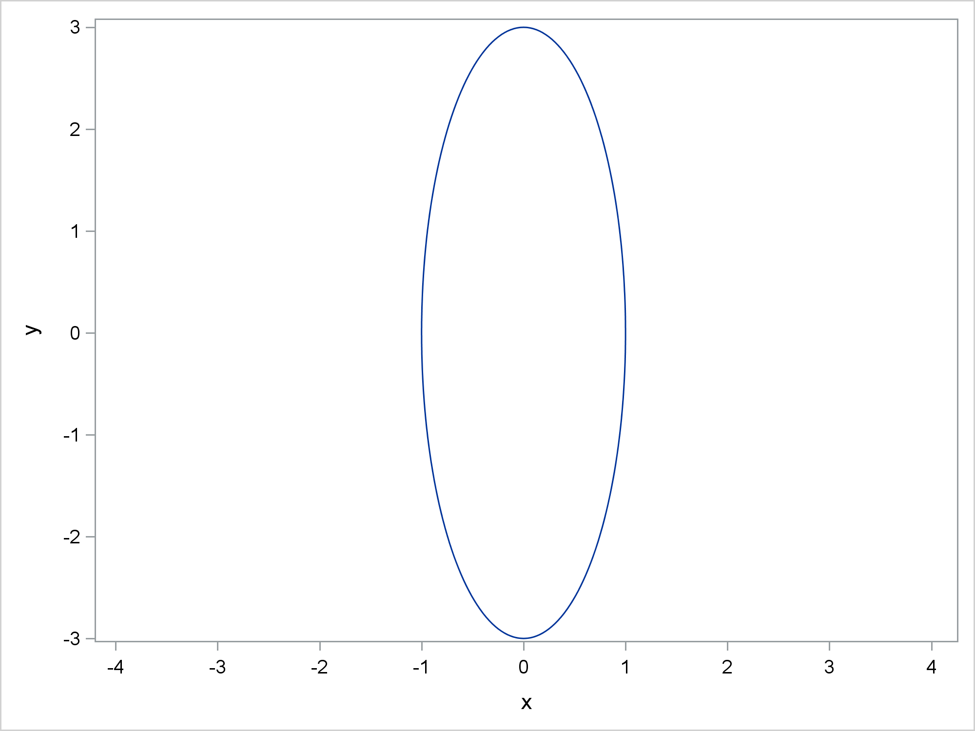
The next step creates coordinates for points on a tall and skinny oval. This is deliberately in contrast to the default graph size, which is wider than it is tall.

data oval(drop=pi tau);
   pi = constant('pi');
   do tau = -pi to pi by pi / 100;
      x = cos(tau);
      y = 3 * sin(tau);
      output;
   end;
run;

The following steps display the oval.

%equate(x, y, data=oval, type=rectangle)
 
%put &minx &maxx &miny &maxy &inc &aspect;
 
proc sgplot data=oval noautolegend aspect=&aspect;
   series  y=y x=x;
   xaxis values=(&minx to &maxx by &inc) &o;
   yaxis values=(&miny to &maxy by &inc) &o;
run;

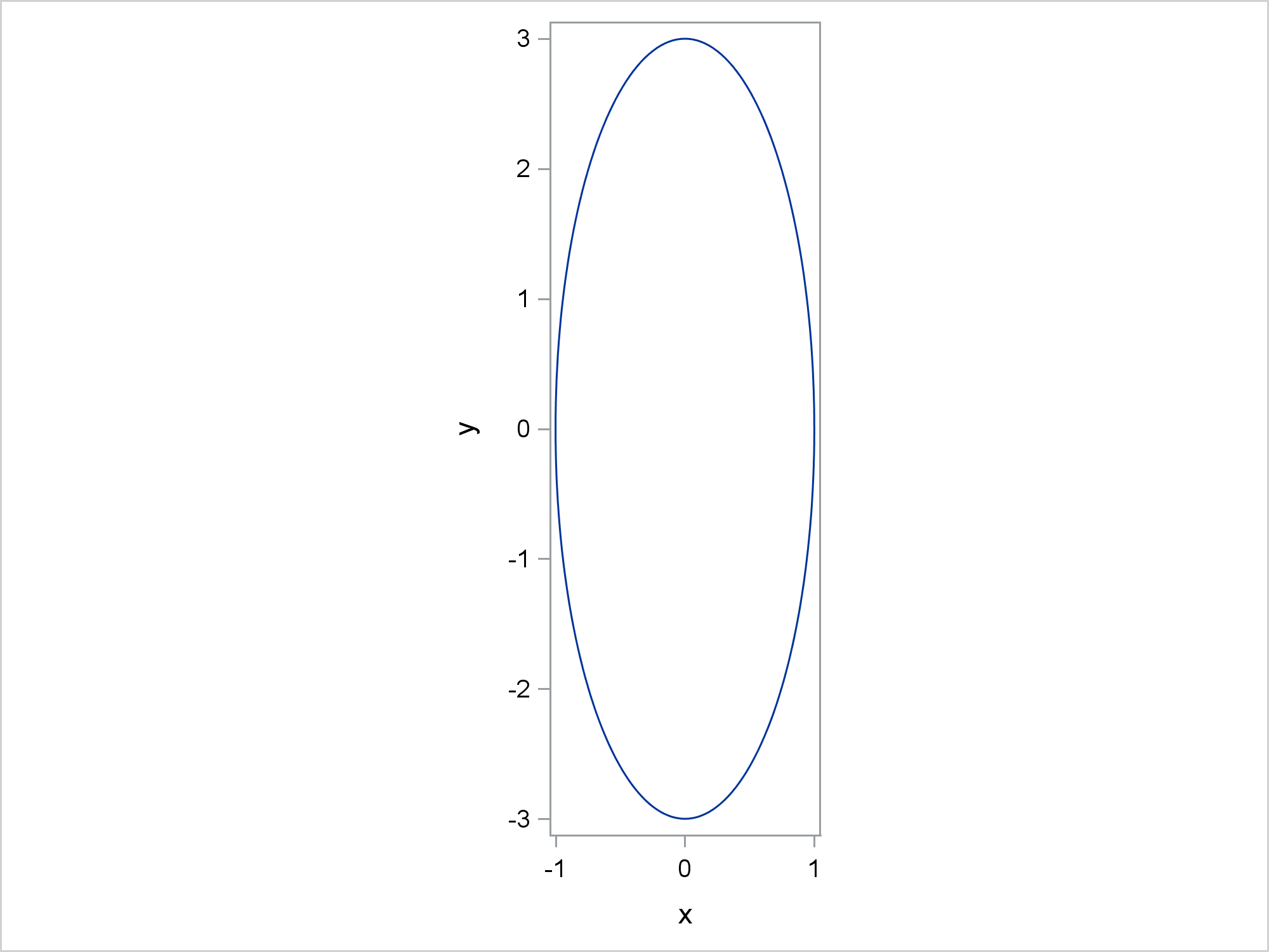
Axes are equated by using an aspect ratio of 3 (which is the factor that was used in the DATA step to scale the height relative to the width).

The following step shows what happens when you specify an aspect ratio of one.

proc sgplot data=oval aspect=1;
   series y=y x=x;
run;

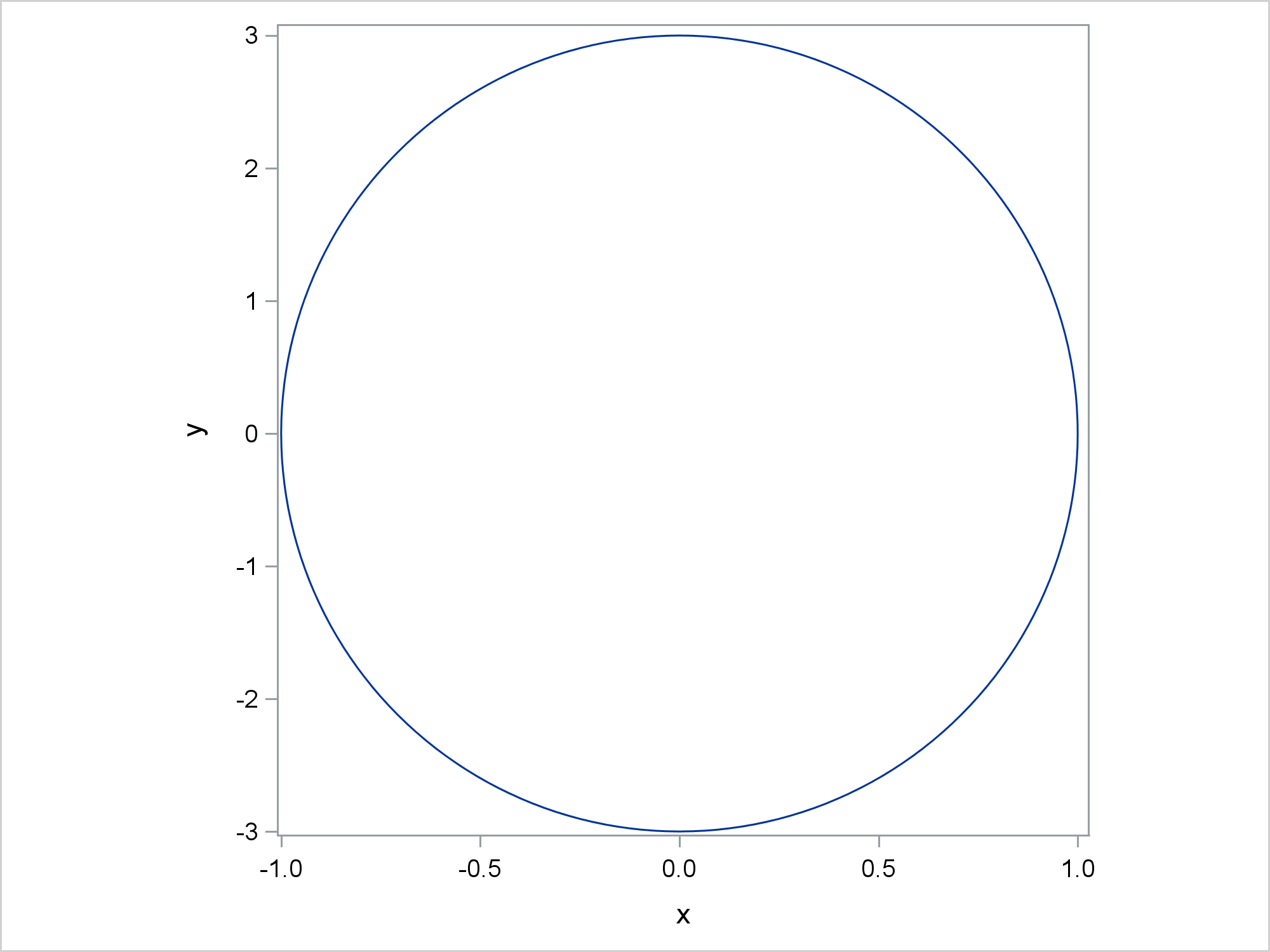
You get what appears to be a circle, but that is not the correct geometry.

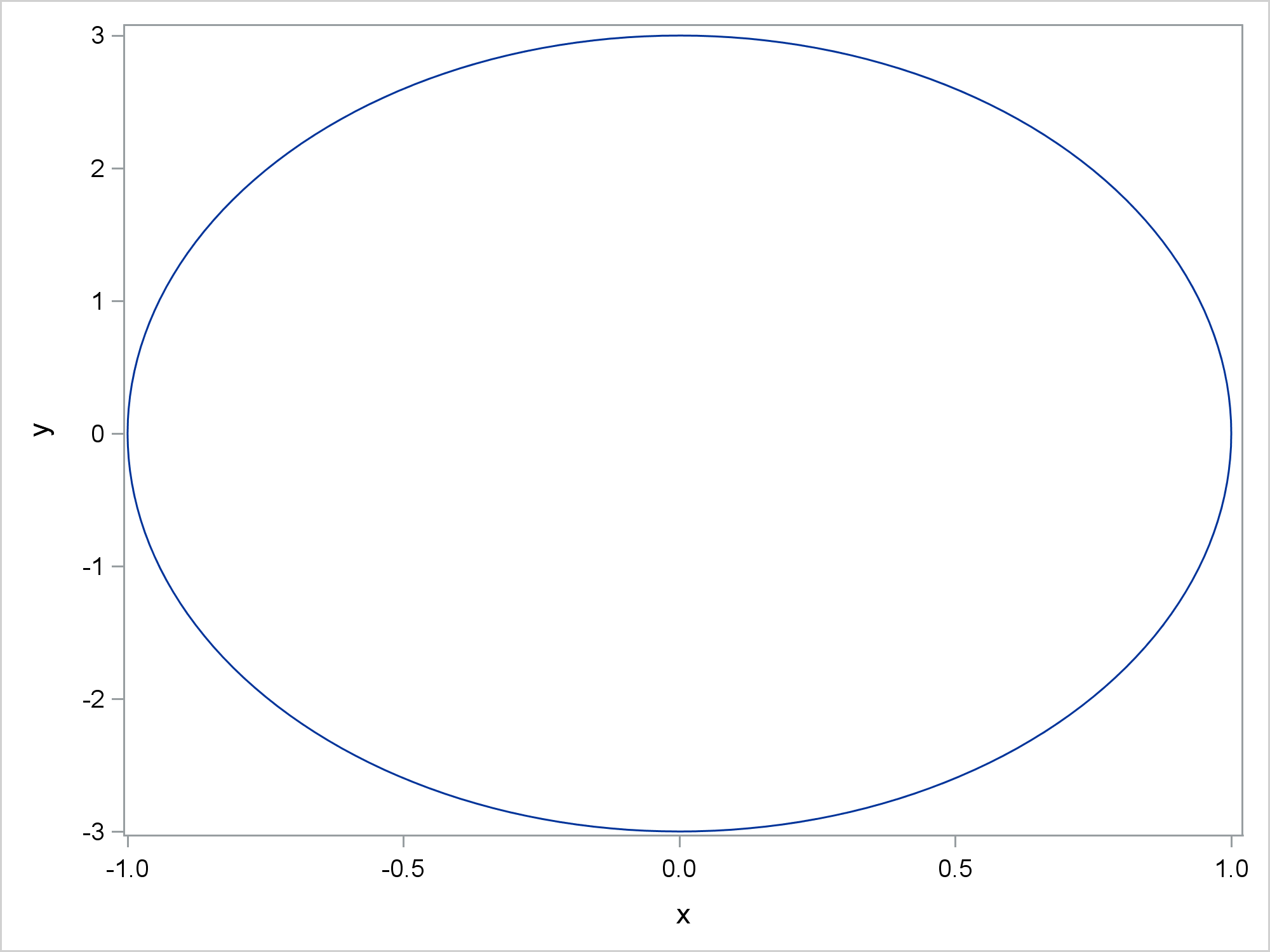
The following shows what happens if you use the default aspect ratio. You get an oval, which again is the wrong shape.

proc sgplot data=oval tmplout='temp';
   series  y=y x=x;
run;

The preceding step also writes the graph template to a file by using the TMPLOUT= option. Readers familiar with my blogs, books, papers, and presentations from the past few years know that I am fond of writing templates to files and then modifying them by using a DATA step. The following step uses PROC SGRENDER and the modified template to create the correct oval.

data _null_;
   infile 'temp';
   input;
   if _n_ = 1 then call execute('proc template;');
   if index(_infile_, 'layout overlay') then
      _infile_ = 'layout overlayequated;';
   call execute(_infile_);
run;
 
proc sgrender data=oval template=sgplot;
run;

These steps work by changing the LAYOUT OVERLAY statement to a LAYOUT OVERLAYEQUATED statement. While this example works perfectly, it also has serious limitations and will not generalize well. I completely replaced the LAYOUT OVERLAY statement that PROC SGPLOT generated. The LAYOUT OVERLAY and LAYOUT OVERLAYEQUATED statements do not have the same options, so you cannot just change the name of the overlay. This also hints at why PROC SGPLOT does not have an EQUATE option. It would not work with many of the currently available PROC SGPLOT options.

If you are serious about equating axes, the GTL has all of the options that you need. PROC SGPLOT with the ASPECT=1 option also equates axes but for more limited displays. By doing some computations and jointly controlling the tick options, offsets, and the aspect ratio, you can use PROC SGPLOT to equate axes for more general data. Of course if you are creating an ad hoc graph and you know the data ranges, you can set your ticks without using a DATA step to find appropriate values.

Code for making shapes like those shown in the first graphs can be found in my free book Basic ODS Graphics Examples or from here.