In SAS, the aspect ratio of a graph is the physical height of the graph divided by the physical width. Recently I demonstrated how to set the aspect ratio of graphs in SAS by using the ASPECT= option in PROC SGPLOT or by using the OVERLAYEQUATED statement in the Graph Template Language (GTL). I mentioned that a unit aspect ratio is important when you want to visually display distance between points in a scatter plot.
A second use of the aspect ratio is when plotting a time series. A time series is a sequence of line segments that connect data values (xi, yi), i = 0..N. Thus a plot involves N line segments, each with a slope and length. In the late 1980s and early '90s, William Cleveland and other researchers investigated how humans perceive graphical information. For a time series plot, the rate of change (slope) of the time series segments is important. Cleveland suggested that practitioners should use "banking to 45 degrees" as a rule-of-thumb that improves perception of the rate-of-change in the plot.
My SAS colleague Prashant Hebbar wrote a nice article about how to use the GTL to specify the aspect ratio of a graph so that the median absolute slope is 45 degrees. Whereas Prashant focused on creating the graphics, the current article shows how to compute aspect ratios by using three banking techniques from Cleveland.
Three computational methods for choosing an aspect ratio
The simplest computation of an aspect ratio is the median absolute slope (MAS) method (Cleveland, McGill, and McGill, JASA, 1988). As it name implies, it computing the median of the absolute value of the slopes. To obtain a graph in which median slope of the (physical) line segments is unity, set the aspect ratio of the graph to be the reciprocal of the median value.
The median-absolute-slope method is a simple way to choose an aspect ratio. A more complex analysis (Cleveland, Visualizing Data, 1993, p. 90) uses the orientation of the line segments. The orientation of a line segment is the quantity arctan(dy/dx) where dy is the change in physical units in the vertical direction and dx is the change in physical units in the horizontal direction.
Cleveland proposes setting the aspect ratio so that the average of the absolute values of the orientations is 45 degrees. This is called "banking the average orientation to 45 degrees" or the AO (absolute orientation) method. Another approach is to weight the line segments by their length (in physical units), compute a weighted mean, and find the aspect ratio that results an average weighted orientation of 45 degrees. This is called "banking the weighted average of the absolute orientations to 45 degrees" or the AWO (average weighted orientation) method.
The AO and AWO methods require solving for the aspect ratio that satisfies a nonlinear equation that involves the arctangent function. This is equivalent to finding the root of a function, and the easiest way to find a root in SAS is to use the FROOT function in SAS/IML software.
For a nice summary of these and other banking techniques, see Heer and Agrawala (2006). However, be aware that Heer and Agrawala define the aspect ratio as width divided by height, which is the reciprocal of the definition that is used by Cleveland (and SAS).
Banking to 45 degrees
To illustrate the various methods, I used the MELANOMA data set, which contains the incidences of melanoma (skin cancer) per one million people in the state of Connecticut that were observed each year from 1936–1972. This is one of the data sets in Visualizing Data (Cleveland, 1993). You can download all data sets in the book and create a libref to the data set directory. (My libref is called vizdata.)
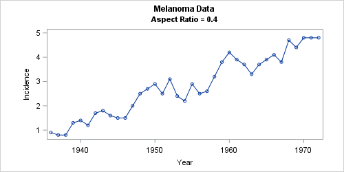
The line plot shows the melanoma time series. The graph's subtitle indicates that the aspect ratio is 0.4, which means that the plot is about 40% as tall as it is wide. With this scaling, about half of the line segments have slopes that are between ±1. This aspect ratio was chosen by using the median-absolute-slope method.
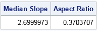
Prashant has already shown how to use the DATA step and Base procedures to implement the median absolute slope method, so I will provide an implementation in the SAS/IML language. The following SAS/IML program reads the data and uses the DIF function to compute differences between yearly values. These values are then scaled by the range of the data. Assuming that the physical size of the axes are proportional to the data ranges (and ignoring offsets and margins), the ratio of these scaled differences are the physical slopes of the line segments. The following computation shows that the median slope is about 2.7. Therefore, the reciprocal of this value (0.37) is the scale factor for which half the slopes are between ±1 and then other half are more extreme. For convenience, I rounded that value to 0.4.
/* Data from Cleveland (1993) */ libname vizdata "C:\Users\frwick\Documents\My SAS Files\vizdata"; title "Melanoma Data"; proc iml; use vizdata.Melanoma; /* see Cleveland (1993, p. 158) */ read all var "Year" into x; read all var "Incidence" into y; close; dx = dif(x) / range(x); /* scaled change in horizontal directions */ dy = dif(y) / range(y); /* scaled change in vertical directions */ m = median( abs(dy/dx) ); /* median of absolute slopes */ print m[L="Median Slope"] (1/m)[L="Aspect Ratio"]; |
Three methods of banking to 45 degrees
I used SAS/IML to implement Cleveland's three techniques (MAS, AO, AWO) and ran each technique on the melanoma data. You can download the complete SAS/IML program that computes the aspect ratios. The following table gives the ideal aspect ratios for the melanoma data as computed by each of Cleveland's methods:
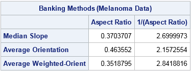
As you can see, the three methods are roughly in agreement for these data. An aspect ratio of approximately 0.4 (as shown previously) will create a time series plot in which the rate of change of the segments is apparent. If there is a large discrepancy between the values, Cleveland recommends using the average weighted orientation (AWO) technique.
The complete SAS program also analyzes carbon dioxide (CO2) data that were analyzed by Cleveland (1993, p. 159) and by Herr and Agrawala. Again, the three methods give similar results to each other.
You might wonder why I didn't choose an exact value such as 0.3518795 for the aspect ratio of the melanoma time series plot. The reason is that these "banking" computations are intended to guide the creation of statistical graphics, and using 0.4 (a 2:5 ratio of vertical to horizontal scales) is more interpretable. Think of the numbers as suggestions rather than mandates. As Cleveland, McGill, and McGill (1988) said, banking to 45 degrees "cannot be used in a fully automated way. (No data-analytic procedure can be.) It needs to be tempered with judgment."
So use your judgement in conjunction with these computations to create time series plots in SAS whose line segments are banked to 45 degrees. After you compute an appropriate aspect ratio, you can create the graph by using the ASPECT= option in PROC SGPLOT or the ASPECTRATIO option on a LAYOUT OVERLAY statement in GTL.
