前回は、SASの「Pipefitter」の基本的な使用方法を紹介しました。続く今回は、基本内容を踏まえ、ひとつの応用例を紹介します。
SAS Viyaのディープラーニング手法の一つであるCNNを「特徴抽出器」として、決定木、勾配ブースティングなどを「分類器」として使用することで、データ数が多くないと精度が出ないCNNの欠点を、データ数が少なくても精度が出る「従来の機械学習手法」で補強するという方法が、画像解析の分野でも応用されています。
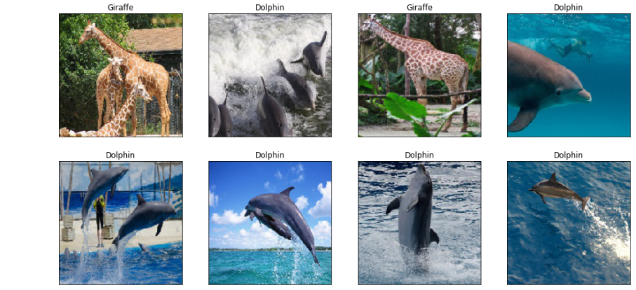
以下は、SAS Viyaに搭載のディープラーニング(CNN)で、ImageNetのデータを学習させ、そのモデルに以下の複数のイルカとキリンの画像をテストデータとして当てはめたモデルのpooling層で出力した特徴空間に決定木をかけている例です。
In [17]: te_img.show(8,4) |
以下はCNNの構造の定義です。
Build a simple CNN model In [18]: from dlpy import Model, Sequential from dlpy.layers import * from dlpy.applications import * In [19]: model1 = Sequential(sess, model_table='Simple_CNN') Input Layer In [20]: model1.add(InputLayer(3, 224, 224, offsets=tr_img.channel_means)) NOTE: Input layer added. 1 Convolution 1 Pooling In [21]: model1.add(Conv2d(8, 7)) model1.add(Pooling(2)) NOTE: Convolutional layer added. NOTE: Pooling layer added. 1 Convolution 1 Pooling In [22]: model1.add(Conv2d(8, 7)) model1.add(Pooling(2)) NOTE: Convolutional layer added. NOTE: Pooling layer added. 1 Dense layer In [23]:model1.add(Dense(16)) NOTE: Fully-connected layer added. Output layer In [24]:model1.add(OutputLayer(act='softmax', n=2)) NOTE: Output layer added. NOTE: Model compiled successfully. In [25]:model1.print_summary() *==================*===============*========*============*=================*======================* | Layer (Type) | Kernel Size | Stride | Activation | Output Size | Number of Parameters | *------------------*---------------*--------*------------*-----------------*----------------------* | Data(Input) | None | None | None | (224, 224, 3) | 0 / 0 | | Conv1_1(Convo.) | (7, 7) | 1 | Relu | (224, 224, 8) | 1176 / 8 | | Pool1(Pool) | (2, 2) | 2 | Max | (112, 112, 8) | 0 / 0 | | Conv2_1(Convo.) | (7, 7) | 1 | Relu | (112, 112, 8) | 3136 / 8 | | Pool2(Pool) | (2, 2) | 2 | Max | (56, 56, 8) | 0 / 0 | | FC1(F.C.) | (25088, 16) | None | Relu | 16 | 401408 / 16 | | Output(Output) | (16, 2) | None | Softmax | 2 | 32 / 2 | *==================*===============*========*============*=================*======================* |Total Number of Parameters: 405,786 | *=================================================================================================* |
このモデル(model1)のPooling層(pool2)で出力した特徴空間に「Pipefitter」を使用して、決定木をかけています。
Extract linear feature from model1 In [56]:x, y = model1.get_features(data=te_img, dense_layer='pool2') In [57]:x, y Out[57]: (array([[ 0., 0., 0., ..., 0., 0., 0.], [ 0., 0., 0., ..., 0., 0., 0.], [ 0., 0., 0., ..., 0., 0., 0.], ..., [ 0., 0., 0., ..., 0., 0., 0.], [ 0., 0., 0., ..., 0., 0., 0.], [ 0., 0., 0., ..., 0., 0., 0.]]), array(['Giraffe', 'Dolphin', 'Giraffe', 'Giraffe', 'Dolphin', 'Giraffe', 'Dolphin', 'Giraffe', 'Giraffe', 'Dolphin', 'Dolphin', 'Dolphin', 'Giraffe', 'Giraffe', 'Giraffe', 'Giraffe', 'Dolphin', 'Dolphin', 'Dolphin', 'Giraffe', 'Dolphin', 'Giraffe', 'Giraffe', 'Dolphin', 'Dolphin', 'Dolphin', 'Dolphin', 'Giraffe', 'Giraffe', 'Giraffe', 'Dolphin', 'Dolphin', 'Dolphin', 'Dolphin', 'Giraffe', 'Dolphin', 'Giraffe', 'Giraffe', 'Giraffe', 'Dolphin', 'Dolphin', 'Giraffe', 'Dolphin', 'Dolphin', 'Dolphin', 'Giraffe', 'Dolphin', 'Dolphin', 'Giraffe', 'Giraffe', 'Giraffe', 'Dolphin', 'Giraffe', 'Dolphin', 'Dolphin', 'Dolphin', 'Giraffe', 'Dolphin', 'Giraffe', 'Dolphin', 'Dolphin', 'Giraffe', 'Dolphin', 'Dolphin', 'Giraffe', 'Dolphin', 'Dolphin', 'Dolphin', 'Dolphin', 'Giraffe', 'Dolphin', 'Dolphin', 'Dolphin', 'Giraffe', 'Dolphin', 'Giraffe', 'Dolphin', 'Dolphin', 'Dolphin', 'Dolphin', 'Giraffe'], dtype=object)) Fit a descision tree using Pipefitter In [58]:import pandas as pd from pipefitter.model_selection import HyperParameterTuning from pipefitter.estimator import DecisionTree, DecisionForest, GBTree In [59]:params = dict(target='label', inputs=[str(i) for i in range(16)]) dtree = DecisionTree(max_depth=6, **params) data = pd.DataFrame(X) data['label'] = y casdata = sess.upload_frame(data) model = dtree.fit(casdata) score = model.score(casdata) score NOTE: Cloud Analytic Services made the uploaded file available as table TMPENYBEVM_ in caslib CASUSER(kesmit). NOTE: The table TMPENYBEVM_ has been created in caslib CASUSER(kesmit) from binary data uploaded to Cloud Analytic Services. Out[59]: Target label Level CLASS Var _DT_P_ NBins 100 NObsUsed 81 TargetCount 81 TargetMiss 0 PredCount 81 PredMiss 0 Event Dolphin EventCount 47 NonEventCount 34 EventMiss 0 AreaUnderROCCurve 0.526283 CRCut 0 ClassificationCutOff 0.5 KS 0.0525657 KSCutOff 0.57 MisClassificationRate 41.9753 dtype: object |
あまり精度がよくありませんが、pool2の出力はかなりスパースっぽいので、それに強い手法の方が良いのかも知れませんね。