Panel data are commonly used in today’s economics research. Panel data regression stands out as a powerful tool that aids in unraveling trends and patterns that evolve over time. This tool is particularly valuable when considering hidden factors in the investigations of cause-and-effect relationships. In this post, you will be given a simple introduction to panel data regression which will showcase the user-friendly CPANEL procedure available in SAS Econometrics. This procedure will be used to explore the intricate dynamics of cigarette demand.

Panel Data Regression

Panel data, also called longitudinal or cross-sectional time series data, is a type of data set that gathers information from multiple observational units over time. Think of it as a collection of snapshots that track changes in various aspects of life. Changes such as annual household income, company performance, or economic conditions like state-level GDP and housing prices.

Panel data regression harnesses this unique data structure to uncover hidden individual (or entity) and time-specific effects. This method helps address issues like causal relationships without needing complicated statistical tools like instrumental variables. It is much more versatile than traditional cross-sectional data analysis techniques. It can even capture broader forms of heterogeneity and dynamic interactions, depending on the specific models used. Next, you will see how to conduct panel regressions for analyzing cigarette demand by using PROC CPANEL.

Cigarette Demand Analysis Using PROC CPANEL

The analysis of cigarette demand, originally explored in Baltagi and Levin (1992), serves as a use case for dynamic panel estimation in Example 10.5 of the PROC CPANEL documentation. This investigation utilizes data from a panel consisting of 46 American states, spanning the years from 1963 to 1992.

The primary variable of interest is the logarithm of real per capita cigarette sales, denoted as LSales. Several factors are considered as potential influencers of sales, including the lag of the outcome variable (LSales_1), the log of the average retail price of a pack of cigarettes (LPrice), the log of real per capita disposable income (LDisp), and the log of the minimum real price in neighboring states (LMin). This last variable serves as a proxy for potential smuggling effects across state borders.

Since all the variables are in logarithmic form, our primary focus of this study lies in identifying the cigarette short-term own-price elasticity (β_LPrice), the income elasticity (β_LDisp), and the cross-price elasticity of cigarette sales within a state concerning the prices in neighboring states, often referred to as the neighboring price elasticity (β_LMin). Furthermore, we can infer the long-term own-price elasticity by using the formula β_LPrice/(1 − β_{LSales_1}), where β_{LSales_1} represents a time discounting factor.

To estimate these elasticities, you can employ PROC CPANEL, which offers a variety of panel data regression techniques. PROC CPANEL is highly performant, thanks to its design to run on a cluster of machines that distribute the data and the computations while exploiting all available cores and concurrent threads.

It's important to note that the selection of these models is primarily for illustrative purposes. In practice, their utilization necessitates sound economic modeling support and appropriate diagnostic tests. Figure 1 provides the SAS code for estimating these models. Figure 2 offers a side-by-side comparison of the results. We will examine these results more closely in the upcoming section.

   proc cpanel data = mycas.Cigar; 
   id State Year;
   model_1: model LSales = LSales_1 LPrice LDisp LMin / pooled; 
   model_2: model LSales = LSales_1 LPrice LDisp LMin / fixone; 
   model_3: model LSales = LSales_1 LPrice LDisp LMin / fixtwo; 
   model_4: model LSales = LSales_1 LPrice LDisp LMin / ranone; 
   model_5: model LSales = LSales_1 LPrice LDisp LMin / btwng; 
   model_6: model LSales = LSales_1 LPrice LDisp LMin / fdone;
   compare / mstat(nobs ncs nts dfe f probf m probm) pstat(estimate stderr probt);
   run;

Figure 1: SAS PROC CPANEL codes estimating various panel data models

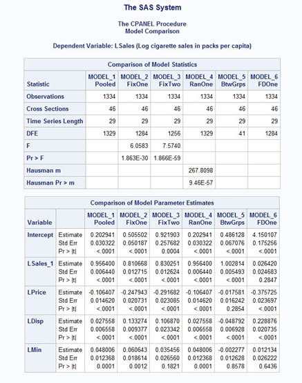
Figure 2: SAS PROC CPANEL regression output comparison

Panel Data Regressions of Cigarette Demand

The one-way error component model is a fundamental framework in panel data analysis:

$y_{it} = x'_{it}\beta + u_i + \epsilon_{it'}$

This is where i indexes the individual and t indexes the time period. $y_{it}$ is the outcome variable, $x_{it}$ is a vector of regressors, $u_t$ is the individual-specific effect, and $\epsilon_{it}$ is an idiosyncratic error term. What sets this model apart from the cross-sectional model is the inclusion of unobservable individual-specific effects, represented by $u_i$. For instance, in a wage regression, $u_i$ could represent an individual worker’s unobserved ability. In a production model, $u_i$ might correspond to a firm-specific productivity factor. In our cigarette demand example, $u_i$ could signify unobservable state-specific factors that remain relatively constant over time, such as regional cultures, demographic characteristics, or geographic attributes. These effects account for variations between individuals that might not be captured by the observed variables. This makes the model particularly suitable for analyzing panel data.

Pooled regression model

The cross-sectional model is indeed a special case of the one-way error component model when the individual-specific effects are assumed to be zero. In panel data analysis, these models are often referred to as pooled regression models. The pooled regression estimator is essentially the traditional Ordinary Least-Squares (OLS) estimator used in cross-sectional models. These models are suitable only when there is compelling evidence that the individual-specific effects are negligible. In our example, this would imply that factors specific to individual states that are constant over time do not significantly influence cigarette sales. This is unlikely to be true.

In Figure 2, you can find the statistics for the pooled regression model under the column labeled MODEL 1. These statistics encompass elasticity estimates and their associated significance levels. Despite neglecting the state and year effects, the signs of these elasticity estimates align with expectations. However, it is worth noting that the short-run price elasticity, which is -0.106, is considerably lower compared to models that take state (and time) effects into account. The long-run price elasticity, -0.106/(1 - 0.956) = -2.410, is much more substantial.

Fixed-effects model

Fixed-effects models are widely favored by economists in panel data analysis because they effectively account for unobservable individual-specific effects without assuming that these effects are uncorrelated with the covariates of interest. The estimator for FE models is often referred to as the within estimator. It essentially applies the OLS estimator to a within-transformation of the one-way error component model, meaning, subtracting the individual means of all the time periods. When there is reason to believe that temporal trends, seasonality, or any unobservable time-varying factors influence the outcome variable, you should consider adding time-specific effects $v_t$ in This leads to a two-way error component model.

In Figure 2, you can find the one-way FE estimates in column MODEL 2 and the two-way FE estimates in column MODEL 3. Compared to the pooled regression estimates, incorporating control for state (and time) effects results in substantially higher short-run price elasticities, -0.248 and -0.292, for one-way and two-way FE, respectively. However, the long-run price elasticities, -1.312 and -1.718, are lower. This suggests that unless the unobserved fixed effects are properly controlled for, they will indeed confound the analysis.

The joint significance of these fixed effects can be further confirmed by observing an F-statistic of 7.57 and a very low p-value in column MODEL 3. Additionally, the F-statistic for the significance of the state effects by themselves is 6.06 with a nearly zero p-value. These results underscore the critical importance of accounting for state and timing factors in the cigarette demand equation.

Random-effects model

Random-effects models are generally more efficient than FE models when the fixed effects are believed to be uncorrelated with the covariates. This efficiency gain makes them particularly popular in microeconomic studies where there are many individuals but relatively few time periods. In such cases, FE models might struggle to capture meaningful time variations due to their reliance on within-individual variation. However, in practice, robustness is frequently favored over efficiency. The strict assumptions required by RE models can limit their applicability. The two-way RE model can also be estimated by using the RANTWO option. We did not include it here since it usually requires even more stringent exogeneity conditions than one-way RE. Consequently, FE models remain more commonly used.

The Hausman test can serve as a specification test to determine whether the assumptions of RE models are appropriate for a given data set. If the test supports the use of RE models, it can provide evidence in favor of this approach. However, it is generally unwise to solely rely on the Hausman test as a decision rule for choosing between RE or FE models. This is because the procedure itself can be biased, as discussed in Hansen (2022). In this example, the Hausman test statistic in column MODEL 4 is 267.81 with an almost zero p-value. This result strongly suggests that FE models are more appropriate for your data set, aligning with the conventional preference for FE models in applied research.

Between-effects model

In contrast to the within estimator used in FE models, which explores variations within individuals, the between-effects estimator focuses solely on variations between individuals. It essentially applies an OLS estimator to the individual averages and assesses the effects of the covariates when they vary between individuals. While the BE estimator is less sensitive to issues related to serial correlation, it is not as commonly employed as FE or RE estimators because it discards all the information across time. As demonstrated from column MODEL 5, the BE model has a much lower degree of freedom, only 41. Therefore, it is consequently less informative.

First-difference model

In addition to the within transformation, first-differencing is another crucial transformation that effectively removes the individual-specific effects. Unlike the within estimator, FD is typically employed when there is a belief that a serial correlation issue exists between the errors. It proves to be efficient when the errors follow a random walk. In column MODEL 6, you can see the estimated own-price and income elasticities by using the FD model. Interestingly, these elasticities are even more substantial in magnitude compared to the within estimators, but the bordering price elasticity is smaller.

Other panel models

Given the results of the joint FE tests and the Hausman test, it seems that the two-way FE model is more suitable for the cigarette demand analysis. Other advanced panel data models can be exceptionally useful for addressing specific challenges in empirical research. IV models are useful when the covariates of interest are endogenous and we have appropriate IVs on hand. Dynamic linear models address the endogeneity issue when lagged outcome variables are included as covariates. Hybrid models, such as Hausman-Taylor and Amemiya-MaCurdy estimations, aim to strike a balance between the consistency of FE models and the efficiency of RE models. More details about these panel models will be discussed in a future post.

Summary

In practice, using pooled regression serves as a useful initial step to gain a preliminary understanding of whether the model is appropriately specified. This is accomplished by examining the signs and magnitudes of the estimates. Conventional practice favors FE models when regressors are suspected to be correlated with unit FEs. Alternatively, RE models can be used for improved efficiency, contingent on the Hausman test not yielding a rejection.

Beyond what we explored so far, PROC CPANEL offers a wealth of features such as restricted estimation and linear hypothesis testing. If you like to learn more about panel data analysis, how to implement these advanced panel methods, and the full capabilities of PROC CPANEL, please refer to the SAS documentation. Moreover, exploring the documented examples can offer valuable hands-on experience. This will significantly assist you on your journey to mastering panel data analysis with PROC CPANEL.