Introduction
Empirical Mode Decomposition (EMD) is a powerful time-frequency analysis technique that allows for the decomposition of a non-stationary and non-linear signal into a series of intrinsic mode functions (IMFs). The method was first introduced by Huang et al. in 1998 and has since been widely used in various fields, such as signal processing, image analysis, and biomedical engineering.[1]
In EMD, the key concepts include non-stationary signals, non-linear signals, and intrinsic mode functions (IMFs). Non-stationary signals are those whose statistical properties, such as mean and variance, change over time. These signals are often encountered in real-world applications and pose challenges for traditional signal processing techniques. Non-linear signals, on the other hand, exhibit complex behavior that cannot be modeled by linear systems. Examples of linear systems for stationary time series include the classical Fourier transform for frequency domain analysis and linear regression, AR, MA, ARMA and ARIMAX models for prediction and forecasting in the time domain.
Intrinsic mode functions (IMFs) are the building blocks of the signal obtained through the EMD process. They represent local oscillatory modes that satisfy specific conditions, allowing for a more intuitive and adaptive representation of the underlying signal. The decomposition into IMFs enables the analysis of non-stationary and non-linear signals in both time and frequency domains, providing valuable insights into their structure and dynamics. An oscillatory mode is a periodic fluctuation or wave-like pattern that appears within a signal. It can be thought of as a continuous function that oscillates between its maximum and minimum values, representing the peaks and troughs of a wave. Visualizing an oscillatory mode, one would see a series of crests and troughs that may vary in amplitude and frequency, yet maintain a consistent oscillatory behavior.
The concept of an envelope is closely related to oscillatory modes. In the context of EMD, an envelope is a smooth curve that surrounds the oscillatory mode, encapsulating the extreme points (peaks and troughs) of the oscillations. There are two types of envelopes: the upper envelope, which connects the local maxima, and the lower envelope, which connects the local minima. Envelopes play a crucial role in the EMD process, as they help to identify and extract the intrinsic mode functions (IMFs) from the original signal. By analyzing the oscillatory modes and their envelopes, it is possible to gain a better understanding of the signal’s structure, its dominant frequencies, and how these components evolve over time.
The EMD algorithm can be described in the following steps:
- Initialize the signal as the input data.
- Identify all local extrema (maxima and minima) in the input data.
- Interpolate between the local maxima and minima to create the upper and lower envelopes, respectively. Typically, cubic spline interpolation is used for this purpose.
- Compute the mean of the upper and lower envelopes, and subtract this mean from the input data to obtain a candidate IMF.
- Check if the candidate IMF satisfies the IMF conditions. If the conditions are met, accept the candidate IMF as an IMF. If the conditions are not met, replace the input data with the candidate IMF and repeat steps 2 to 5.
- Subtract the accepted IMF from the original input data to obtain the residuals.
- If the residuals are not negligible, consider it as the new input data and repeat steps 2 to 6. Otherwise, stop.
In the Empirical Mode Decomposition (EMD) algorithm, determining whether the residuals is negligible or not is typically based on either a predefined stopping criterion or a user-defined threshold. Here are some common ways to decide if the residue is negligible:
- Visual inspection: One can inspect the residuals visually and decide whether it contains any meaningful oscillatory patterns or not. If it appears as random noise or a constant trend, then the residue can be considered negligible.
- Iteration limit: Sometimes, a maximum number of iterations is set as a stopping criterion. If the algorithm reaches this limit, the residuals is considered negligible, and the decomposition process is stopped.
- Variance criterion: A common stopping criterion is to calculate the variance of the residuals and compare it to the variance of the original signal or the previously extracted IMF. If the ratio of these variances falls below a certain threshold, the residuals is considered negligible.
- Power threshold: Another approach is to calculate the L2 norm of the residuals and compare it to the L2 norm of the original signal or the previously extracted IMF. If the ratio of these energies falls below a certain threshold, the residuals is considered negligible.
These methods can be used individually or in combination to determine if the residuals is negligible or not. It is important to note that the choice of the stopping criterion may influence the results of the EMD algorithm, and it is often problem-specific.
Applications
Because of EMDs ability to analyze non-stationary and non-linear signals, it has been applied in many contexts and domains. Here are three examples of the application of EMD:
- Biomedical Signal Processing: EMD has been widely applied in the analysis of biomedical signals such as Electroencephalogram (EEG), Electrocardiogram (ECG), and Electromyogram (EMG) signals. It helps in detecting abnormal patterns, diagnosing diseases, and understanding the underlying physiological mechanisms. In Martis, et. al. the authors propose a novel methodology for automatically classifying EEG signals of normal, inter-ictal, and ictal epileptic subjects using EMD.[3] The study utilizes EMD to extract intrinsic mode functions (IMFs) from the EEG signals, which are then transformed using the Hilbert transform to obtain amplitude and frequency modulated (AM and FM) frequencies. Features such as spectral peaks, spectral entropy, and spectral energy in each IMF are extracted and fed into decision tree classifiers for automated diagnosis. The authors compare the performance of two types of decision tree classifiers: classification and regression tree (CART) and C4.5. The highest average accuracy (95.33%), sensitivity (98%), and specificity (97%) are achieved using the C4.5 decision tree classifier. This methodology is now ready for clinical validation on larger databases and has the potential to be deployed for mass screening in the diagnosis of epilepsy.
- Mechanical Fault Diagnosis: EMD has been employed in the field of mechanical engineering for fault diagnosis, especially in rotating machinery. It assists in identifying faults in gears, bearings, and other mechanical components by analyzing the vibration signals generated during operation. Zhang and Zhou present a comprehensive fault diagnosis method for rolling bearings.[5] The method includes two parts: the fault detection and the fault classification. In the stage of fault detection, a threshold based on refined composite multiscale dispersion entropy (RCMDE) at a local maximum scale is defined to judge the health state of rolling bearings. If the bearing is in fault, a generalized multi-scale feature extraction method is developed to fully extract fault information by combining empirical mode decomposition (EMD) and RCMDE. The IMFs from EMD are used as features which are fed into a random forest model to classify faults versus normal operations. The results of the experiment indicate that the proposed method can fully extract the fault information of vibration signals.
- Financial Time Series Analysis: Nava, et. al. introduce a multistep-ahead forecasting methodology that combines empirical mode decomposition (EMD) and support vector regression (SVR).[4] The methodology is based on the idea that forecasting is simplified when EMD-decomposed time series are used as input for SVR. The authors compare the performance of their methodology with benchmark models commonly used in the literature. The EMD technique decomposes non-stationary data into a finite set of intrinsic mode functions (IMFs) and the residuals. These IMFs are locally stationary, have simpler structures, and are associated with oscillations within a characteristic time scale range. The authors successfully demonstrate that IMFs are better suited for forecasting than the original time series. They test both univariate and multivariate EMD-SVR forecasting schemes and evaluate their performance on intraday data from the SP 500 index. The results suggest that the multivariate EMD-SVR models perform better than benchmark models, with the most significant improvements observed for longer-term horizons. High-frequency IMFs contribute to short-term forecasting, while low-frequency components are better for long-term forecasting. The authors acknowledge that there is scope for further refining the methodology, such as improving the selection of input vector and SVR parameters, and better handling of boundary values and noise propagation. Overall, the study demonstrates the feasibility of using EMD for forecasting purposes and the effectiveness of the proposed EMD-SVR forecasting methodology in predicting the Standard & Poor’s 500 Index from 30 seconds to 25 minutes ahead.
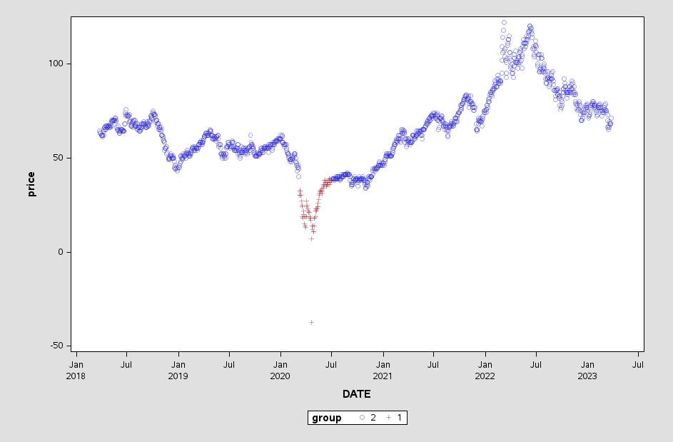
The applications discussed above demonstrate the versatility and effectiveness of the Empirical Mode Decomposition (EMD) technique in various fields, such as automated detection of epilepsy using EEG signals, fault diagnosis of rolling bearings, and financial time series forecasting. In light of these successful applications, it is worth exploring the application of EMD to other time series data as well. The SAS/IML CALL EMD routine provides a convenient tool for computing the empirical mode decomposition of a time series, enabling you to further investigate the potential benefits of EMD in different contexts. In the following example we will investigate the use of EMD on simulated oil price data, specifically West Texas Intermediate Oil(WTI). The time series of the WTI oil prices can be visualized below:
SAS/IML CALL EMD Example
In this example, the Empirical Mode Decomposition (EMD) method analyzes simulated West Texas Intermediate (WTI) Oil Price Data. Specifically, the CALL EMD subroutine within the SAS/IML software performs the decomposition process.[2] This technique will enables you to extract Intrinsic Mode Functions (IMFs) from the data, which can then be used to uncover underlying trends, cycles, and other significant components present in the WTI oil price time series.
In addition to the decomposition process, we will hint at methodologies for forecasting future values of the Intrinsic Mode Functions (IMFs) obtained through EMD. By generating accurate forecasts for the IMFs, you can subsequently predict future oil prices, thereby enabling more informed decision-making in the energy market. The insights gained from this analysis could prove valuable for industry stakeholders, policymakers, and financial investors as they navigate the complexities of the oil market and its potential future trends. In this example the following steps will be discussed:
- Preprocessing the simulated time series.
- Perform Empirical Mode Decomposition (EMD) to obtain Intrinsic Mode Functions (IMFs) and residual.
- Split the data into temporally contiguous training and test sets based on a specified date.
- Perform time series forecasting of a single IMF using the proc tsmodel procedure.
The full source code for this article can be found on GitHub.
Preprocessing
The SAS code below performs two main operations on a dataset containing daily WTI oil prices. The first part of the code uses the TIMESERIES procedure to process the dataset wti_oil_prices and add rows for any missing dates, creating an output dataset called wti_oil_prices_fill. It sets the ID variable DATE at daily intervals, ensuring that the dataset is consistently spaced in time. The TIMESERIES procedure specifies no accumulated values, sets missing values for added rows and formats the DATE variable with the DATE9. format. The variable of interest in this step is PRICE, which represents the WTI oil prices.
The second part of the code uses the EXPAND procedure to interpolate missing values in the dataset created in the previous step. The input dataset is wti_oil_prices_fill, and the output dataset is wti_oil_prices_fill_int. The EXPAND procedure uses the JOIN method to interpolate the missing values for the PRICE variable and creates a new variable, PRICE_INT, containing the interpolated values. The ID variable for this step is DATE, which helps the procedure understand the structure of the data. Overall, the code handles missing values and interpolates the WTI oil prices dataset to create a more complete and consistent dataset for further analysis.
proc timeseries data = wti_oil_prices out = wti_oil_price_fill; id date interval = day accumulate = none setmiss = missing format = date9.; var price; run; proc expand data=wti_oil_price_fill out=wti_oil_price_fill_int; convert price=price_INT / method=join; id DATE; run; |
Empirical Mode Decomposition
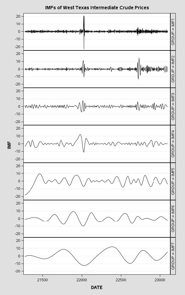
In the PROC IML code, the input data (dates and interpolated oil prices) are read from the wti_oil_prices_fill_int dataset into two vectors, DATES and OIL_PRICES. Afterward, the CALL EMD subroutine is called with the specified options to decompose the oil prices into Intrinsic Mode Functions (IMFs) and a residual component. The obtained IMFs are illustrated in a panel series plot to visualize the IMFs over time. The code then combines the dates, IMFs, original oil prices, and the residual component into a single matrix called OUTPUT, which is subsequently used to create a new dataset wti_oil_price_IMF.
options orientation = portrait; ods graphics on / reset width=600px height=1000px border=off ANTIALIASMAX=50100; proc iml; use wti_oil_price_fill_int; read all var {DATE} into dates; read all var {price_INT} into oil_prices; close wti_oil_prices_interp; optn = {10 1 .01 .001}; call EMD(IMF, residual, oil_prices,optn); title "IMFs of West Texas Intermediate Crude Prices"; call panelSeries(dates, IMF, {'IMF1','IMF2','IMF3',...,'IMF7'}) grid="y" label={"DATE" "IMF"} NROWS=7; ndates=nrow(dates); output=shape(1,ndates,10); output[,1]=dates; output[,2:8]=IMF; output[,9]=oil_prices; output[,10]=residual; varnames={'DATE' 'IMF1' 'IMF2' 'IMF3' ... 'IMF7' 'price_INT' 'RESIDUAL'}; create wti_oil_price_IMF from output[colname=varnames]; append from output; close; quit; |
You can visualize the historical IMFs in the following panel:
IMF Forecasting
The TSMODEL code below fits a moving average (MA) model on the first intrinsic mode function (IMF1) extracted from the decomposed West Texas Intermediate (WTI) oil price series, and then generates forecasts. The MA orders are defined using an array (ma) with three elements: 1, 2, and 3. The ARIMA model specification (mySpec) is then configured with these MA orders using the AddMAPoly() method, while the NOINT and METHOD options are set to 1 (no intercept) and ’CLS’ (conditional least squares), respectively. Lastly, the model forecasts, parameter estimates, and statistics are collected using TSMFor, TSMPEst, and TSMSTAT objects, respectively.
proc tsmodel data=CASUSER.TRAIN outobj=(outStat=CASUSER.OUTEST_IMF1(replace=YES) outFcast=_tmpcas_.outFcastTemp(replace=YES) parEst=CASUSER.OUTFOR_IMF1(replace=YES) ) seasonality=7; id DATE interval=Day FORMAT=_DATA_ nlformat=YES; var IMF1; require tsm; submit; declare object myModel(TSM); declare object mySpec(ARIMASpec); rc=mySpec.Open(); array ma[3]/nosymbols; ma[1]=1; ma[2]=2; ma[3]=3; rc=mySpec.AddMAPoly(ma); rc=mySpec.SetOption('noint', 1); rc=mySpec.SetOption('method', 'CLS'); rc=mySpec.Close(); rc=myModel.Initialize(mySpec); rc=myModel.SetY(IMF1); rc=myModel.SetOption('lead', &lead); rc=myModel.SetOption('alpha', 0.05); rc=myModel.Run(); declare object outFcast(TSMFor); rc=outFcast.Collect(myModel); declare object parEst(TSMPEst); rc=parEst.Collect(myModel); declare object outStat(TSMSTAT); rc=outStat.Collect(myModel); endsubmit; run; |
The next step in forecasting WTI oil prices involves leveraging the intrinsic mode functions (IMFs) extracted from the empirical mode decomposition (EMD) of historical data. By considering both the actual historical IMFs and projected future IMFs, we can incorporate these insights as exogenous regressors in a predictive model. This approach allows for a comprehensive understanding of the underlying components and trends that drive oil price fluctuations. By utilizing the IMFs as exogenous inputs, the model can better capture nonlinear and non-stationary patterns that traditional time series models might struggle with. Consequently, this method aims to enhance the accuracy and reliability of WTI oil price forecasts, providing valuable information for stakeholders and decision-makers in the energy industry.
Conclusion
The next step in forecasting WTI oil prices involves leveraging the intrinsic mode functions (IMFs) extracted from the empirical mode decomposition (EMD) of historical data. By considering both the actual historical IMFs and forecasted future IMFs, you can incorporate the IMFs as exogenous regressors in a predictive model. This approach allows for a comprehensive understanding of the underlying components and trends that drive oil price fluctuations. Since the empirical mode decomposition (EMD) technique decomposes the original time series into a set of IMFs, it isolates the intrinsic oscillations and trends present in the data. This allows for the identification and separation of various time-varying patterns, which are often responsible for the non-stationarity in oil price series. By incorporating these IMFs as exogenous inputs, the model is better equipped to account for the dynamic nature of oil price fluctuations. As a result, forecasting models becomes more robust and reliable, successfully handling non-stationarity and providing more accurate predictions.