The image action set in SAS Viya Machine Learning provides tools to import and preprocess images. These processed images can then be imported into the deep learning action set for training machine learning classification models. These two action sets together can create a comprehensive end-to-end image classification machine learning pipeline.

In this post, we will demonstrate how to utilize SAS Viya Machine Learning to train a convolutional neural network that can accurately detect patients with COVID-19 by using the transfer learning technique. As a reference, we will follow the methodology established in the study by Tuan D. Pham.

Data sets

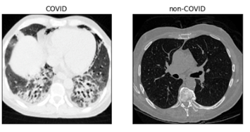
For this demonstration, we will use CT images from 80 COVID and 542 non-COVID subjects from Harvard Dataverse, Mendeley Data, and the Cancer Imaging Archive. All the COVID subjects have a confirmed positive COVID-19 diagnosis. The CT images for the COVID subjects and the six non-COVID subjects were originally 3-D DICOM files with 100+ image slices. The CT images for the 536 non-COVID subjects are in PNG format. So all 3-D DICOM files were converted to 2-D PNG format. Images that do not include enough lung regions were removed from any further analysis.  In total, 1392 COVID and 1120 non-COVID CT 2-D images were used to train the classification model. Figure 1 shows an example of CT images for a COVID and a non-COVID subject.

Importing and preprocessing data in SAS Viya

To begin our pipeline, we first import all the images by using the image action set. Note that ‘decode’ must be set to ‘False’ for further deep learning analysis.

   inputimg=s.CASTable(name='inputimg',replace=True)
   s.image.loadimages(casout=inputimg,
                  path='COVID_chest_CT/covid_classify/',
                  caslib='dlib',
                  recurse=True,
                  labellevels=-1,
                  decode=False,
                  addcolumns=['width','height'])

Next, all the input images are resized to 224x224. They are normalized to a range of 0 to 255 by using the MINMAX normalization. These functionalities are available in the processImages action.

   processed=s.CASTable(name="processed")
   s.image.processImages(images=dict(table=inputimg),
                     steps=[
                         dict(step=dict(steptype='RESIZE',type='BASIC',height=224,width=224)),
                         dict(step=dict(steptype='NORMALIZE', type='MINMAX',alpha=0 ,beta=255))
                     ],
                     decode=False,
                     casOut=processed)

Further, the processed images are converted to ImageTable by using the DLPy ImageTable class, as shown here. In this way, all the processed images can be sent to DLPy for further deep learning analysis.

   my_images=ImageTable.from_table(processed, image_col='_image_', label_col='_label_')

Once the processed images are converted to ImageTable, they are then split into the training, validation, and test sets. Here, 64%, 16%, and 20% of the images are used for training, validation, and testing, respectively. The DLPy library is applied to implement the data splitting in a Pythonic way.

    train_val, test_table=two_way_split(my_images, test_rate=20, seed=123)
    train_table, val_table = two_way_split(train_val, test_rate=20, seed=123)

Building a classification model in SAS Viya

Given that our classification task is relatively simple, it is necessary to utilize a deeper model to learn the complex representations of COVID-19. We must do this while avoiding overfitting. In this regard, the ResNet-50 model has been shown to be effective, achieving 93% accuracy according to Pham. However, training a model from scratch often requires a large amount of data to achieve satisfactory results. To mitigate this issue, we can utilize a pretrained model on the ImageNet data set to leverage the learned representations from this data set.

To load a pretrained ResNet50, we can utilize the DLPy library and specify certain model specific parameters such as the number of classes, the channels of the input data, and offsets, for example. The pretrained weights should be stored in an h5 file and specified when instantiating the ResNet50_Caffe class.

   pre_train_weight_file=os.path.join(PRE_TRAIN_WEIGHT_LOC, 'ResNet-50-model.caffemodel.h5')
   from dlpy.applications import resnet
   from dlpy.model import AdamSolver,VanillaSolver, Optimizer
   from dlpy.lr_scheduler import ReduceLROnPlateau, CyclicLR, PolynomialLR
   resModel=resnet.ResNet50_Caffe(s, 
                                 model_table='ResNet50_Caffe', 
                                 n_classes=2,
                                 n_channels=3, 
                                 width=224, 
                                 height=224, 
                                 scale=1,
                                 random_crop=None,
                                 pre_trained_weights=True, 
                                 pre_trained_weights_file=pre_train_weight_file,
                                 include_top=False)

Finally, the fit function from the DLPy library is applied to fit the model. Here, VanillaSolver was specified along with a learning rate scheduler of the Cyclic Learning Scheduler class. The optimizer was defined with the VanillaSolver, a log level of 2, a max_epochs of 10, and a mini_batch_size of 4.

   lrs=CyclicLR(s, train_table, 4, 1.0, 1E-4, 0.01)
   solver=VanillaSolver(lr_scheduler=lrs)
   optimizer=Optimizer(algorithm=solver, log_level=2, max_epochs=20, mini_batch_size=4)
   resModel.fit(data=train_table,
             optimizer=optimizer, 
             gpu=dict(devices=[2]),
             n_threads=4,
             valid_table=val_table,
             log_level=2)

Evaluating a classification model in SAS Viya

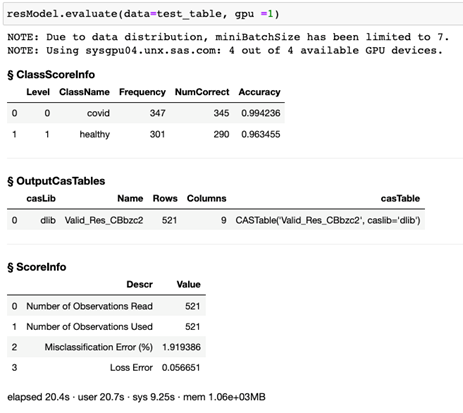
Now that we have built and trained the model, we can use the model to score the test data set. This is done by using the evaluate function from the DLPy library. The response is shown in Figure 2. For the given test images, our model classifies subjects with COVID with 99.4% accuracy. It classifies non-COVID subjects with 96.3% accuracy.

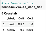
We can further visualize the performance of our classification model by creating a confusion matrix by using the valid_conf_mat function from the DLPy library. The response is shown in Figure 3. The confusion matrix is used to compare the predicted classes of true positives (column 1, row 1), false negatives (column 2, row 1), false positives (column 1, row 2), and true negatives (column 2, row 2). In this case, out of the validation data set, one subject with COVID was misclassified as non-COVID. Nine non-COVID subjects were misclassified as COVID subjects.

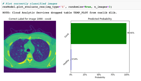
The image classification results can be plotted as shown in Figures 4 and 5. Here, we utilize the plot_evaluate_res function from DLPy to display a plot with an image that was correctly classified (actual class = predicted class, or img_type = ‘C’), along with a predicted probability bar chart for this given image.

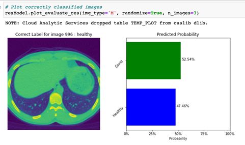
By specifying the img_type to ‘M’, the code displays a plot with an image that was incorrectly classified (actual class not equal to predicted class, or img_type = ‘M’), along with a predicted probability bar chart for this image as shown in Figure 5.

Further, the heat_map_analysis function from DLPy can be applied to use color to indicate the regions of interest that provide the most useful information to the model, letting it determine a distinction of each class. We can use these regions of interest to understand how reliable our model’s predictions are and why the model struggles with misclassified images. The resulting figures are shown in Figures 6 and 7.

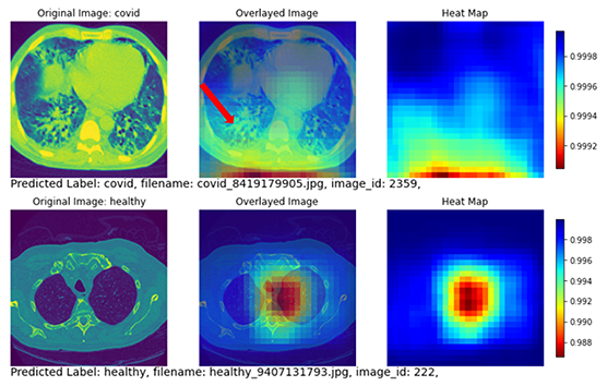
Figure 7 shows two subjects with correctly classified classes. The top row shows a COVID subject with the disease region mostly focused on the posterior lung. The heat map also highlights the posterior lung as the region of interest (yellow and red regions in the heat map). The bottom row shows a non-COVID subject with no diseased region appearing in the lung. The heatmap highlighted the central part of the lung without focusing on any specific areas.

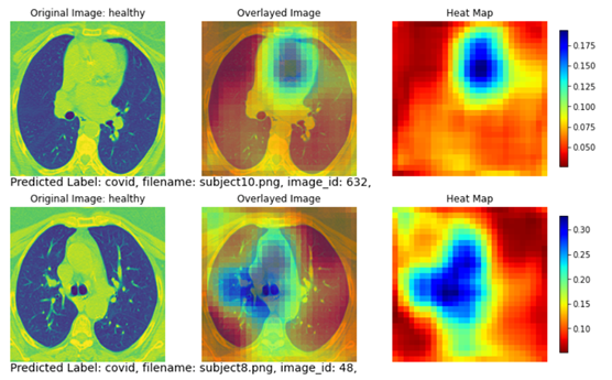
Figure 7 shows two subjects with misclassified classes. The top row shows a healthy subject that is misclassified as a COVID subject. Although this subject does not have apparent disease areas in the lung, the classification model looked through the entire lung area (yellow and red regions covering nearly the entire heat map) and decided there is a higher likelihood that this subject is a COVID subject. The predicted probability is 51.24% for COVID and 48.76% for non-COVID.

The bottom row in Figure 8 shows another healthy subject that is misclassified as a COVID subject. Similar to the example on the top row, no apparent disease areas are present in the lung. Therefore the heatmap covers the whole image without focusing on a specific lung region. Like the subject on the top row, the classification model determined there is a higher chance that this subject is a COVID subject. The predicted probability is 54.75% for COVID and 45.25% for non-COVID.

Discussion

The use of the optimizer and learning rate scheduler was crucial in achieving exceptional results after only three epochs. Non-adaptive optimizers (vanilla solver in this work), as demonstrated in the study by Wilson et al., tend to generalize better than adaptive optimizers. This is likely because non-adaptive optimizers do not make changes to their learning rate based on the current state of the model, which can prevent overfitting. On the other hand, adaptive optimizers adjust the learning rate based on the model's performance. This can lead to better performance on the training data but potentially poorer generalization to unseen data.

In addition to the use of a non-adaptive optimizer, the inclusion of a cyclic learning rate scheduler has been shown to significantly increase the speed of training in computer vision tasks. This is accomplished by periodically varying the learning rate over the course of training. In turn, this can help prevent the model from getting stuck in suboptimal configurations and facilitate faster convergence. Given the importance of both training speed and generalization capabilities for the model, the combination of these two elements is an optimal choice for achieving exceptional results.

Summary

In this post, we examined the process of training a pretrained convolutional neural network to classify COVID-19 CT scans by using SAS Viya Machine Learning, leveraging its learned representations to achieve exceptional results. The classification model in this work was built upon a pretrained ResNet-50 model. It achieved a 99.4% accuracy rate in classifying COVID subjects and a 96.3% accuracy rate in classifying non-COVID subjects. The classification model can accurately focus on the lung regions with disease infection on the COVID CT images.

While examining the misclassified subjects, it was found that most of them are non-COVID subjects that were misclassified as COVID subjects. Among these misclassified non-COVID subjects, all of them do not have apparent disease regions in the lung. Although the classification model assigns a COVID class to these subjects, all of them only have a slightly higher predicted probability for the COVID class compared to the non-COVID class. Overall, SAS Viya Machine Learning provides a high degree of experimental design freedom and versatility in achieving our COVID classification model in this work.

Acknowledgment

Special thanks to Sebastian Alberto Neri for his contribution to this work. Sebastian is a rising senior student at Monterrey Institute of Technology in Mexico. He joined the Computer Vision team in August 2022 as an intern. This work is part of Sebastian’s internship project.