Firms typically face a heterogeneous set of customers. Characteristics such as age, gender, income, genetics, and so on, vary among individuals. Such variability can affect how customers respond, for example, to a treatment or to a price increase. Understanding individual responses to treatments or marketing offerings are therefore crucial for informed individualized pricing (treatment) decisions. PROC DEEPPRICE offers a flexible framework for specifying and estimating individual responses to treatments.
PROC DEEPPRICE enables you to specify treatment effects as unknown functions of observed individuals’ characteristics. It uses Deep Neural Networks to estimate unknown functions. Such a rich and flexible approach to accounting for individual variability in treatment responses has the advantage of capturing complex forms of heterogeneity, even with large data sets. It enables firms to determine, for example, what types of consumers are price sensitive. And they can leverage such individual differences for personalized prices. In addition to the individual effects, PROC DEEPPRICE also provides estimates for quantities of interest such as average treatment effects.
PROC DEEPPRICE also enables you to perform policy analysis comparing outcomes under various hypothetical treatments. It can answer questions such as “What is the best pricing strategy to optimize revenue?” or “What is the suitable dose to attain a desired response?”
Personalized pricing for revenue optimization
Let’s look at an example of how an online media company can offer targeted discounts through personalized pricing to optimize revenue.
The data set is provided by the Microsoft research project ALICE. For more details, see Example 15.1 in the PROC DEEPPRICE documentation. The data set has 10,000 simulated observations that represent users’ personal characteristics. These include age, income, and account age. Also taken into account is users’ online behavior history, including previous purchases and previous online times per week. The treatment variable, price, is the price the customer was exposed to during the discount season. The outcome variable, demand, is the number of songs that the customer purchased during the discount season. Table 1 shows the names of the variables that are used in the model, along with their type and definition.
| Name | Variable Type | Definition |
| demand | Outcome | Number of songs purchased during the discount season |
| price | Treatment | The price that the user was exposed to during the discount season |
| account_age | Covariate | User’s account age |
| age | Covariate | User’s age |
| avg_hours | Covariate | Average number of hours user was online per week in the past |
| days_visited | Covariate | Average number of days user visited website per week in the past |
| friend_count | Covariate | Number of friends user connected to in account |
| has_membership | Covariate | Whether user has membership |
| is_US | Covariate | Whether user accesses website from the United States |
| songs_purchased | Covariate | Average number of songs user purchased per week in the past |
| income | Covariate | User’s income |
Table 1: Model variables
The following SAS code estimates the effect of price on the demand for songs and the details of the estimation used later for policy evaluation.
/*--- Estimate the treatment effect and save the estimation details ---*/ ods output ParameterEstimates=ParameterEstimates; proc deepprice data=mycas.new_pricing_sample; id id; tmodel price = account_age age avg_hours days_visited friends_count has_membership is_US songs_purchased income / dnn=(nodes=(32 32 32 32) train=(optimizer=(miniBatchSize=500 regL1=0.0001 maxEpochs=32000 algorithm=adam) nthreads=20 seed=12345 recordseed=67890)); model demand = account_age age avg_hours days_visited friends_count has_membership is_US songs_purchased income / dnn=(nodes=(32 32 32 32) train=(optimizer=(miniBatchSize=500 regL1=0.001 maxEpochs=32000 algorithm=adam) nthreads=20 seed=12345 recordseed=67890)); infer out=mycas.oest outdetails=mycas.odetails; score outt=mycas.outtdata outa=mycas.outadata outb=mycas.outbdata; run; |
Shown below is the estimated average slope. It represents the average (over all the users) price coefficient in the demand model. It is negative, as expected, and statistically significant.
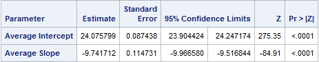
Heterogeneity in user-specific price sensitivities
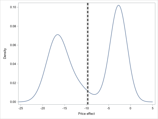
The average price effect aggregates individual-specific effects over all the users. The distribution of the individual-specific price effects can be visualized by creating a density plot of the individual price effects by using the following SAS code. The results are shown in Figure 1, which also shows the average price effect and its 95% confidence interval represented by the vertical band.
data _null_; set ParameterEstimates; if (parameter='Average Slope') then do; call symputx('mean_beta', estimate); call symputx('lowerCL_beta', LowerCL); call symputx('upperCL_beta', UpperCL); end; run; proc sgplot data=odetails noautolegend; density _beta_ / type=kernel lineattrs=(pattern=solid); refline &lowerCL_beta/ axis=x lineattrs=(thickness=1 color=grey pattern=dash); refline &upperCL_beta/ axis=x lineattrs=(thickness=1 color=grey pattern=dash); refline &mean_beta/ axis=x lineattrs=(thickness=10 color=lightgray) transparency=0.6; refline &mean_beta/ axis=x lineattrs=(thickness=3 color=black pattern=dash); xaxis label='Price effect' values=(-25 to 5 by 5); run; |
Clearly, there are substantial differences among individual price effects. The average price effect is about -10, but there are two distinct groups of users. One group has a prominent peak at around -2 and the other at -17.
A useful quantity of interest is the price elasticity of demand, which measures the percentage change in the number of songs purchased when there is a 1% increase in price. In general, demand decreases when the price increases for most products (the price effect is negative). However, the amount by which demand decreases is greater for some products than for others. PROC DEEPPRICE output is used to compute individual-specific elasticities. Their distribution is shown by the density plot in Figure 2.
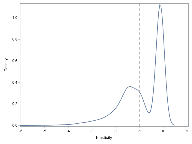
Figure 2 shows a rich heterogeneity in price elasticities. There are clearly two groups of users. One group is exclusively price insensitive with elasticity around zero. The second group has a higher variance and includes highly price-sensitive users. An average estimate of the price coefficient would have masked this heterogeneity, which is important for setting personalized prices.
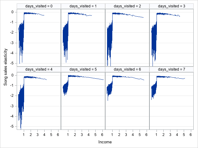
The variability of price elasticities with selected users’ characteristics (income and days_visited) is shown in Figure 3. There is a remarkable heterogeneity among users. Low-income users (income <1) are more sensitive to a price increase. Their price elasticities range from –5 to –1. This means that if the price goes up by 1%, the number of songs purchased falls by 1% to 5%. This is compared to around 0.15% for higher-income users. Moreover, low-income users who visited the website less often in the past (days_visited <5) are even more price-sensitive than low-income users who visited the website more often (days_visited >4). The latter group has a price elasticity between –2 and –1, compared to a range of –5 to –1 for the former. This information is important for targeting users with a price discount.
Translating heterogeneity in price effects into personalized prices
Given the estimated individual-specific price effects, the online media company seeking to maximize revenue can set optimal prices for each user as \(price_*^i =-\frac{\alpha(x_i)}{2\beta(x_i)}\). These prices guarantee the maximum revenue and are highly personalized, but they can exceed the original prices. The above variability in price elasticities suggests that the online media company might want to consider a price discount that targets a specific group of users. Table 2 shows the observed pricing policy price, the revenue-maximizing policy s1, as well as six other discounted policies for comparison.
| Policy | Definition | Description |
| price | Current prices (baseline price * small discount) | Observed |
| s0 | Offer no one a discount | Simple benchmark |
| s1 | Optimal personalized revenue- maximizing prices | Estimated: \(price_*^i =-\frac{\alpha(x_i)}{2\beta(x_i)}\) |
| s1d | Discounted optimal personalized prices | s1d = s1 if s1 <=1 ; 1 otherwise |
| s2 | Offer low-income users who spend on average less than 5 days a week on the website a 10% discount | Elasticity related |
| s3 | Offer everyone a 5% discount | Simple benchmark |
| s4 | Offer low-income users who spend on average less than 5 days a week on the website a random discount (5%, 10%, 15%, 20%, 25%, or 30%) | Elasticity related |
| s5 | Offer every user a random discount (5%, 10%, 15%, 20%, 25%, or 30%) | Simple benchmark |
Table 2: Pricing policies
Policy evaluation and comparison
We observed the number of songs purchased at the observed prices and can compute the corresponding revenue per user, but we wish to learn what the revenue per user would be if the online media company had set a different price. For example, consider the eight different price strategies described in Table 2. We wish to compare each of the seven hypothetical pricing policies with the observed prices and to determine which policy generates the most revenue. The SCORE and INFER statements in PROC DEEPPRICE enable you to do that after estimating the price effects and saving the details of the estimation.
The following SAS code evaluates and compares each of the policies s0, s1, s1d, s2, s3, s4, and s5 to the observed policy price.
proc deepprice data=mycas.discountPolicy; id id; infer out=mycas.oest2 outdetails=mycas.odetails2 policy=(price s0 s1 s1d s2 s3 s4 s5) policyComparison=(base=(price) compare=(s0 s1 s1d s2 s3 s4 s5)); score int=mycas.outtdata ina=mycas.outadata inb=mycas.outbdata; run; |
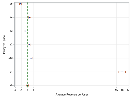
The results of the policy comparison are plotted in Figure 4. Each of the hypothetical policies is compared to the observed policy price, and each blue-filled marker represents the revenue difference between each policy and price. The green dotted line represents a revenue difference of zero. Markers on the left to the green line represent policies that are worse than price, and those on the right represent policies that are better than price. Refer to Table 2 for the definition of each policy. The optimal personalized revenue-maximizing prices policy, s1, is the best.
However, because prices under s1 can exceed the original prices, the discounted optimal personalized policy, s1d, is more meaningful. The policy s1d and the policies that target price-sensitive users (s2 and s4) are comparable and are better than price. The policy s0 (offer no user a discount) is equivalent to price. Policies that offer every user a discount (s3 and s5) are worse than price, with s5 being the worst.
Conclusion
PROC DEEPPRICE offers a unified framework for estimating heterogeneous causal effects of continuous treatments and performing policy analysis. Its flexibility has enabled us to specify individual price effects as a function of individuals’ characteristics. The estimated individual price effects were then translated into individualized prices. These were used, along with other hypothetical pricing strategies, to show how the online media company can set user-specific prices to achieve maximum revenue. Or show how to adopt discount policies that target a specific group of users to increase revenue.
The analysis presented assumed that the variable price is exogenous. That is, the price variable is not correlated with the error term in the demand model. This assumption might not hold. In that case, PROC DEEPPRICE can still be used and will require the user to provide an instrumental variable.