Authors: Bahar Biller and Xi Jiang
The ability to identify the key drivers of risk is critical for the successful management of all supply chains. A technique enabling the identification of risk drivers in complex supply chains is sensitivity analysis. Specifically, sensitivity analysis (SA) quantifies the impact of variations in system inputs on key performance indicators (KPIs). Thus, when coupled with supply chain KPI prediction, SA is the tool used to empower supply chain practitioners to identify the key supply chain risk drivers. It further enhances the understanding of supply chain performance. It also helps determine what drives the cost and presents guidance on input management.
Use case: semiconductor manufacturing plant (fab)
Consider a semiconductor wafer fab with the process-flow illustrated in Figure 1. The process consists of two basic steps, Diffusion and Lithography. Each contains multiple sub-steps. In this wafer fab, which operates 24/7, cassettes are released at a constant rate of one per hour. The raw cassette begins at the Clean station. It passes through a full cycle of diffusion and lithography steps multiple times before leaving the system. The times spent at Oxidize, Coat, and Stepper are assumed to be deterministic. The processing times at Clean, Load, Unload, and Develop stations (marked with a star in Figure 1) are variable. Their distribution types and mean values are presented in Table 1.
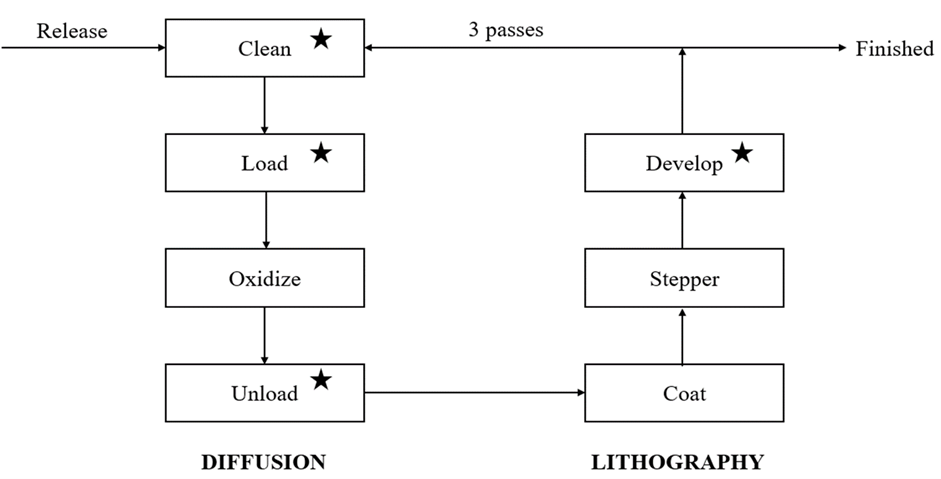
A KPI of interest in this use case is the flow time. Flow time is the amount of time it takes to complete the manufacturing processes from the release of a cassette to the finish. We mimic how cassettes flow through this manufacturing facility with the help of a stochastic simulation. We use the simulated process-flow output data to obtain the risk profile of the flow time. Then we execute the simulation for 900 replications, each with a run length of seven days (168 hours).
| Station | Machine Count | Distribution | Mean (Hours) |
| Clean | 9 | Exponential | 1.821 |
| Load | 1 | Lognormal | 0.283 |
| Oxidize | 11 | Constant | 2 |
| Unload | 1 | Lognormal | 0.283 |
| Coat | 7 | Constant | 1.5 |
| Stepper | 6 | Constant | 1.5 |
| Develop | 3 | Gamma | 0.494 |
Table 1 Semiconductor manufacturing plant inputs
After quantifying the risk profile of the flow time KPI, it is important to study its sensitivity to means and standard deviations of uncertain processing times. As an example, if the mean processing time spent at the Clean station decreased by one hour, what would be the impact on the mean flow time? Or what would be the impact if the standard deviation of the cleaning time decreased by one hour? A way to answer these questions is by using a specific type of SA technique. This is known as the local sensitivity analysis.
Sensitivity analysis: going beyond the traditional manufacturing KPI prediction
Inputs of a simulation model represent real-world uncertainty at its most basic level. In our semiconductor manufacturing plant simulation, inputs include the number of machines available at each step. Also included are the processing times of these machines (that is, Machine Count, Distribution, and Mean (Hours)). Processing time can be deterministic or variable due to lack of information, errors of measurement, or estimation errors. Uncertainties in the inputs (for example, processing times) will imply uncertainty in the outputs (for example, flow time). SA studies how the model output responses are affected by the inputs to better understand system performance, quantify risk, or indicate where input change or management might be desirable.
Depending on the type of input and the goals of the analysis, SA methods can be grouped into two categories, global SA and local SA. Further subdivisions can exist within each. Here we focus on the local SA:
- Global SA imposes a distribution on each input factor based on prior knowledge or data. Then, the measured output variability caused by variation in the input factors (over the entire range of the possible values) is apportioned to each input factor as a measure of its contribution to output uncertainty. Consequently, measures of global SA provide qualitative guidance as to which inputs to control or study to reduce their uncertainty. And which inputs are not significant sources of output uncertainty to reduce the risk in estimating the output.
In the case of the semiconductor wafer fab use case, global SA would apply if we know their ranges, for example, 1<α<10 and 10<β<15 but don’t know the values of the shape (α) and rate (β) of the gamma distribution modeling the processing time at the Develop station. Global SA would tell you which of these two parameters matters more qualitatively. However, if the goal were to conduct a what-if scenario analysis, then local SA, instead of global SA, would have to be used.
- Local SA focuses on the impact of small perturbations of the input on the outputs. This is often in the form of a partial derivative of the output with respect to the input. Because this type of sensitivity analysis applies only to an infinitesimal perturbation around the nominal setting, it is truly local. Consequently, it identifies the key risk drivers in the current system state and allows management to focus on a few of the many uncertain inputs. Through local SA, at SAS, we equip our customers with the ability to quantify the expected change in the mean KPI per unit change in the mean or standard deviation of the corresponding uncertain input. Within the context of the semiconductor wafer fab use case, we could compute the change in mean flow time in response to a change of one hour in the mean or standard deviation of the processing time spent at any of its stations.
However, doing so is not a straightforward task when there are multiple ways to achieve a change in mean (μ) or standard deviation (α) because different changes in the input parameter vector might lead to the same change in μ or α but different changes in the expected flow time. For example, this is the case with the gamma-distributed processing time at the Develop station. Fortunately, there exists a new family of local sensitivity measures that quantify the sensitivity of the output mean to a change in the input’s mean or standard deviation along a specified direction in the input-parameter space. A mathematical description of this quantification is available in a technical paper recently featured on the SAS Science Community. Next, we discuss the results of the local SA implementation in SAS for our semiconductor manufacturing use case.
Results: flow time risk profile and sensitivity measures
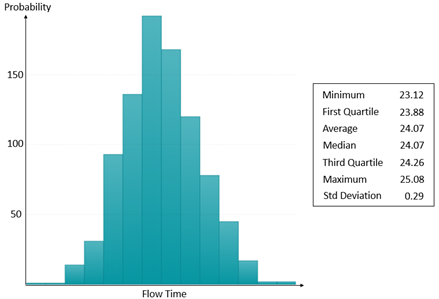
As illustrated in Figure 2, we have the analysis of the 900-replication simulation output data results in the flow time risk profile. It shows that the expected flow time is 24.07 hours with a standard deviation of 0.29 hours. This implies that the average flow time falls between 24.05 hours (that is., 24.07-1.96*0.29*(900)-1/2) and 24.09 hours (that is, 24.07+1.96*0.29*(900)-1/2) for 95% of the time. However, there is a 25% chance that the flow time falls below 23.88 hours as well as a 25% chance that the flow time exceeds 24.26 hours.
Next, we ask the following question. If we could improve the performance of a single station, which one of the Clean, Load, Unload, and Develop stations should we focus our effort on? Quantitatively, we pose eight different questions, two of which are as follows for the Clean station:
- If mean cleaning time decreased by one hour, what would be the impact on mean flow time?
- If the standard deviation of the cleaning time decreased by one hour, what would be the impact?
We repeat these questions for the processing times of the remaining three (Load, Unload, and Develop) stations. What is important to note here is that, instead of conducting eight different simulation experiments, the answers to these questions are obtained all at once by applying the local SA technique to the simulation output data. These have already led to the risk profile in Figure 2. We visualize the resulting sensitivity measures in Figure 3. These results have been obtained from the local sensitivity analyzer we have developed by using SAS OPTMODEL together with SAS NLMIXED, REG, and IML procedures.

Figure 3 contains two plots, each of which presents sensitivity measures using tornado plots. Plot A presents the mean flow time sensitivity to the mean processing time. Plot B summarizes the mean flow time sensitivity to the standard deviation of processing time. Furthermore, an illustration of each measure is accompanied by an error bar showing the standard deviation interval on the estimated sensitivity.
We immediately see from Plot A that Develop and Clean are the two manufacturing steps that would reduce the mean flow time the most with improved mean processing times. A one-hour decrease in the Develop processing time would lead to a reduction of 3.6 hours in the mean flow time. A one-hour decrease in the Clean processing time would lead to a reduction of 3.2 hours in the mean flow time. On the other hand, improving the processing times at Load and Unload stations has a much smaller impact on flow time.
Plot B hints that mean flow time is not sensitive to the change in the standard deviations of the processing times at the Load and Unload stations. Therefore, these two stations are excluded from Plot B. It also shows that an hour reduction in the standard deviation of the processing time at the Develop station decreases the mean flow time by eight hours.
The same improvement in the processing time of the Clean station is expected to reduce the mean flow time by approximately three hours. On one hand, these results indicate the importance of quantifying the impact of input uncertainty on the flow time KPI. On the other hand, they provide us the last piece of information that will answer the question posed earlier. If there would be an opportunity to improve the processing time of a single manufacturing step in the fab, we would recommend restricting focus to the Develop station.
Summary
This post discusses the critical role of sensitivity analysis in supply chain risk analysis. As an example, we use a simplified semiconductor manufacturing plant. It helps explain that sensitivity quantification is critical. It answers what-if questions for business systems with complex process flows and exposure to high levels of input risk. The sensitivity measures suggest smart resource management and effort allocation strategies that are both time and cost-efficient for customers that might face supply chain disruptions brought on by the pandemic. They further provide guidance in minimizing risk and improving productivity as an important component of manufacturing analytics. At SAS, we are committed to equipping our customers with the power of advanced analytics to help them succeed on this journey.