In this post, I will introduce the new SASEBEA interface engine in SAS^® Econometrics, which provides easy access to the US Bureau of Economic Analysis (BEA) economic statistics data. Forecasting and econometric models are often improved by incorporating additional variables into the model. SAS/ETS^® includes nine access engines that enable you to query, process, and retrieve free and proprietary time series data directly from third-party data providers. The access engines afford you the convenience of directly converting imported data to SAS data sets. The SASEBEA interface engine was introduced in the 2021.1.1 release and completed in the 2021.2.2 release of SAS^® Viya^® 4.

The BEA produces some of the world’s most closely watched statistics. This includes the US gross domestic product, better known as GDP. They also provide state and local numbers plus foreign trade and investment stats and industry data.

There are a total of 12 distinct data set names. Each requires its own unique set of options to request data using the SASEBEA interface engine. Figure 1 shows the list of those data sets.

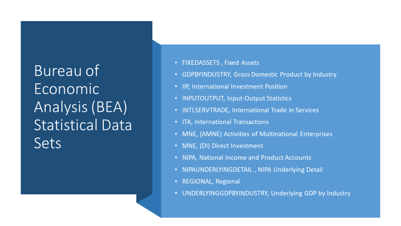
The 12 data sets fit into four categories: industry, national, international, and regional. The industry data sets include the GDP by Industry, Underlying GDP by Industry, and Input-Output Statistics. For national, we have the National Income and Product Accounts (NIPA Tables), the NIPA Underlying Detail Accounts, and the Fixed Assets Accounts. The international data sets include the International Trade in Services, the International Transaction Accounts (ITA), International Investment Position (IIP), Activities of Multinational Enterprises (AMNE), and Direct Investment (DI). For the regional category, we have one data set, Regional.

For accessing any of the BEA data sets, you will need an API key. Once you have an API key, you have free access to the BEA’s public data.

Accessing the GDPBYINDUSTRY data

With the GDP statistics, you can examine how fast the US economy is growing. You can also compare each state’s economy and determine which industries are growing and which are slowing down. The county GDP stats can be used to analyze how the economic output is distributed across the nation. They can also help to identify the local areas most in need of economic development. They also help study which development strategies work best. Counties can use these GDP numbers to attract investors. Businesses can use them to make decisions about new locations and investments.

There are three closely watched price indexes:

• The personal consumption expenditures price index measures prices paid by consumers and reflects changes in what they’re buying.
• The gross domestic purchases price index measures prices paid throughout the US economy, including prices paid for imports.
• The GDP price index measures goods and services produced in the United States, including those exported abroad.

Here’s a quick example to show how easy it is to use the SASEBEA engine to access the GDP data.

GDP example

You simply specify a few options in the SASEBEA LIBNAME statement, such as SETNAME=, FREQ=, INDUSTRY=, TABLEID=, and YEAR= options, as shown in the following SAS code:

   options validvarname=any;
   libname beagi sasebea ""
         setname=GdpByIndustry
         TableID='7'
         user='XXXXXXXX-XXXX-XXXX-XXXX-XXXXXXXXXXXX'
         freq=a
         industry='7,71,71AS'
         outjson=Mgdp7
         year=all
         format=json;
   data work.myMgdp7; set beagi.Mgdp7; run;
   proc contents data=work.myMgdp7; run;
   proc print data=work.myMgdp7; run;

This example requests data from the BEA data set named GdpByIndustry for TABLEID=7. It is named “Components of Value Added by Industry as a Percentage of Gross Domestic Product (A)”. The industries, specified by INDUSTRY=’7,71,71AS’, are:

• 7: Arts, entertainment, recreation, food services (A) (Q)
• 71: Arts, entertainment, recreation (A) (Q)
• 71AS: Performing arts, spectator sports, museum, and related activities (A) (Q)

The FREQ= option requests annual data, and the YEAR= option requests all available years. The FORMAT= option requests the data to be in a JSON file, and the OUTJSON= option specifies the name of the JSON file containing the requested data. The LIBNAME statement options specify all the parameters necessary to request the GDP data to be retrieved from the BEA. The DATA step names the SAS output data set that contains the requested data. The SET statement specifies that SAS reads the JSON data named ‘Mgdp7’.

Note that the libref BEAGI is used in the SET statement to indicate that the SASEBEA LIBNAME statement with the libref BEAGI is to be used to request the data. This example program returns 23 years of data and 13 variables. The CONTENTS procedure gives a list of variables and their attributes. You can use the myMgdp7 table in the same way as you use any other SAS table, like printing it by using the PRINT procedure. The physical path given on the SASEBEA LIBNAME statement must be a writable folder location because the engine uses that location to read the data into SAS.

Input-Output statistics

The Input-Output accounts (I-O) provide a detailed view of the interrelationships between US producers and users. Businesses, national policymakers, state and local governments, academics, and others rely on analytical tools derived from the I-O framework, such as:

• Trade in Value Added (TiVA) Statistics trace global value chains through direct and indirect US trade partners, improving understanding of the US role in international trade.
• Computable General Equilibrium (CGE) Models anticipate the response of the economy to changes in policy, changes in technology, and other external shocks.
• Regional Impact Analysis Models show the local impact of a specific project or event like a strike or natural disaster.

To access the Input-Output data set, the options for the SASEBEA libname statement are even simpler than the GDP example. You only need to specify the options: SETNAME=InputOutput, TableID=, USER=, OUTJSON=, YEAR=, and FORMAT=JSON.

NIPA tables

Let’s turn our attention now to the National data, the NIPA (National Income and Product Accounts) tables, and the NIPA Underlying Detail statistics. These data include personal income numbers, the income that is left (after taxes) that is available for American consumers to either spend or save. The nation’s personal saving rate is the percentage of disposable income that is saved. These numbers can give insight into Americans’ financial health or the future of consumer spending. They are used to determine the allocation of hundreds of billions of federal dollars to states and local areas each year. Policymakers use estimates of wages and salaries to project federal budgets and Social Security trust fund balances. Other data on noncash income, such as employer contributions to workers’ health care coverage, help complete the picture of labor costs.

Corporate profit numbers contained in these data are closely watched economic indicators. These quarterly data include US corporations’ combined earnings from current production, with breakdowns for durable goods, manufacturing and retail trade. These data help the government monitor the effects of policy changes and help predict how much tax corporations will owe. They are also important for forecasting spending on factories and equipment.

To access the NIPA data set, you only need to specify the SETNAME=NIPA, TableName=, USER=, FREQ=, OUTJSON=, YEAR=, and FORMAT=JSON options.

Another National data set, Fixed Assets, only needs you to specify the SETNAME=FixedAssets, TableName=, USER=, OUTJSON=, YEAR=, and FORMAT=JSON options.

International Transaction Accounts

Let’s take a look at the international data. This is best known for capturing the trade gap, the difference between US exports and imports. These data include estimates of trade deficits or surpluses that the US has with other nations. It also shows what is being traded with whom. The balance of payments between the United States and other countries are important economic indicators. They are part of the International Transaction Accounts (ITA) data set.

To access the ITA data set, you only need to specify the SETNAME=ITA, INDICATOR=, AREAORCOUNTRY=, USER=, FREQ=, OUTJSON=, YEAR=, and FORMAT=JSON options.

International Trade in Services

The international trade in services statistics is largely based on data collected by the BEA’s confidential business surveys. Detailed statistics on annual international services are provided by the International Trade in Services data set (IntlServTrade). It includes the services provided by the local affiliates of multinational companies. Trade direction and affiliations are included in the options.

To access the IntlServTrade data set, you need to specify the SETNAME=IntlServTrade, TYPEOFSERVICE=, AFFILIATION=, AREAORCOUNTRY=, USER=, TRADEDIRECTION=, OUTJSON=, YEAR=, and FORMAT=JSON options.

International Investment Position

Next, let’s take a closer look at the international trade and investment numbers. Trade numbers help policymakers and the public understands how exports and imports affect US businesses, jobs, and growth. These data can come into play when negotiators make trade agreements and when businesses need to know more about export markets. The International Investment Position (IIP) data set is a statistical balance sheet that shows the difference between US residents’ foreign financial assets and liabilities at the end of each quarter.

To access the IIP data set, you need to specify the SETNAME=IIP, TYPEOFINVESTMENT=, COMPONENT=, USER=, FREQ=, OUTJSON=, YEAR=, and FORMAT=JSON options.

Direct Investment and Activities of Multinational Enterprises

The last international data set is the MNE data set. It houses both Direct Investment (DI) data and Activities of Multinational Enterprises (AMNE). Direct Investment statistics are used to understand the scale of foreign ownership in the United States and how it affects the economy. These data can show trends in offshoring by US companies. It also shows the effects of tax changes and other laws on multinational enterprises. Researchers use them to study the factors that influence foreign investment decisions, and the factors that affect jobs, wages, and tax revenues at home and abroad.

To access the MNE data set for direct investment statistics (DI), you need to specify the SETNAME=MNE, COUNTRY=, CLASSIFICATION=, DIRECTIONOFINVESTMENT=, FOOTNOTES=, INDUSTRY=, SERIESID=, USER=, OUTJSON=, YEAR=, and FORMAT=JSON options.

To access the MNE data set for activities of multinational enterprises (AMNE), you need to specify the SETNAME=MNE, COUNTRY=, CLASSIFICATION=, DIRECTIONOFINVESTMENT=, FOOTNOTES=, INDUSTRY=, NONBANKAFFILIATESONLY=, OWNERSHIPLEVEL=, SERIESID=, STATE=, USER=, OUTJSON=, YEAR=, and FORMAT=JSON options.

Regional Accounts

The Regional Accounts are the final data set we will look at. There are many uses for regional data. The Federal government uses regional income and product estimates to distribute funds to states for programs such as the FY2020 Federal Health and Wellness ($547.9 billion), the FY2020 Federal Funds Distribution to the Department of Agriculture, and to programs administered by the Departments of Commerce, Economic Development, Education, and Health and Human Services. Twenty states have set constitutional or statutory limits on state government revenues (taxes) or spending that are tied to BEA state personal income or one of its components. Other consumers of the Regional data are businesses, trade associations, labor organizations in market research, researchers in applied economics, and the  National Oceanic and Atmospheric Administration (NOAA) for coastal area statistics.

To access the regional data set, you need to specify the SETNAME=REGIONAL, TABLENAME=, LINECODE=, GEOFIPS=, USER=, OUTJSON=, YEAR=, and FORMAT=JSON options.

Using CAS with the SASEBEA engine

To use a CAS in-memory table for our output data, SASEBEA requires three additional options: GOCAS=, CASLIB=, and OUTCAS= options. When GOCAS=ON is specified, the SASEBEA engine assumes there is an active CAS session running before the SASEBEA LIBNAME statement is used. The CASLIB= option names the CAS library where the in-memory CAS table is stored, and CASOUT= options specify the name of the in-memory CAS table that is created when the JSON data from the BEA are read into SAS. Below is an updated version of the GDP example with these three options added.

   libname beagi sasebea ""
      gocas=on caslib=casuser casout=myCasMgdp7
      setname=GdpByIndustry
      TableID='7'
      user='XXXXXXXX-XXXX-XXXX-XXXX-XXXXXXXXXXXX'
      freq=a
      industry='7,71,71AS'
      outjson=Mgdp7
      year=all
      format=json;

The resulting CAS table is named myCasMgdp7. You can use this CAS table now, just like you use any other CAS table.

Three additional ETS engines, SASEMOOD for Moody’s Analytics Data, SASEFRED for Federal Reserve Economic Data, and SASEWBGO for World Bank Group Open Data, use the same three options to enable these time series data to be stored for use in CAS.

Other powerful tools for exploring the BEA statistical data

The BEA supports online interactive tables called ‘Itable’ for all of these data sets. There are helpful links to research papers and background information that support the methods used for these statistics. There is a Tools tab on the BEA web page listing the available exploratory tools. The News tab, the Research tab, and the Resources tab are also worthy of investigation. Make sure you visit the Learning Center under the Resources tab.

Conclusion

Whether you are interested in industry, national, international, or regional statistics, the US Bureau of Economic Analysis has significant historical and current time series data for enhancing your econometric modeling. In addition to the SASEBEA engine, interfaces to other econometrics data include SASEFAME, SASEHAVR, SASEXCCM, SASEFRED, SASEXFSD, SASERAIN, SASENOAA, SASEQUAN, SASEWBGO, and SASEMOOD.  For SAS users, the new SASEBEA interface engine provides seamless access to all 12 of the BEA data sets. This adds yet another data source for enhancing your analyses.