
State space models (SSMs) have long been used in a wide variety of fields like econometrics, signal processing, and environmental science. They are used to analyze data generated in a sequential fashion such as time series, panels of time series, and longitudinal data. The CSSM procedure in SAS® Econometrics, the SAS® Viya® version of the SSM procedure in SAS/ETS®, provides a comprehensive set of tools for analyzing such sequential (streaming) data. Scoring is an important new feature in the 2021.1.6 release of PROC CSSM. Scoring can be used for efficient, model-based scenario analysis and stability monitoring of an ongoing data stream. This post discusses this new scoring feature.
Scoring with state space models
Scoring is evaluating a previously fitted model at some new predictor setting. For example, a bank might score a new loan application by applying a rule that is based on a previously fitted logistic regression model. You might also want to use SSMs for scoring. Because of the sequential nature of the observation process, it is important to realize that the scoring process for an SSM is inherently different from the scoring process for a model that is based on independent observations. Examples would be simple linear regression or logistic regression.
Think of a sequential data process like a long-running TV series, with a new episode every week. Watching the series for some time and learning about the main characters and their relationships to each other is akin to fitting a model to the initial portion of a sequential data stream. After you have watched some episodes, you can make educated guesses about the subsequent plotline. You can also imagine different ways the series could play out, while still being consistent with the storyline.
For sequential data, this process of forecasting and what-if analysis, based on the fitted model and ever-increasing history, is called scoring. Additionally, the scoring process enables you to monitor an ongoing observation process for additive outliers (that is, one-off observations) and structural breaks such as shifts in the mean level or other patterns.
PROC CSSM
The scoring process requires a model that is a good fit for the initial portion of the data stream. After a suitable model is fitted, a score store is created. The score store contains sufficient information for you to forecast subsequent observations of the data stream, without having access to its history. If scenario analysis is the only goal, this initially created score store is all that is needed for scoring different future scenarios. On the other hand, if the goal is to perform stability monitoring of the ongoing data stream, the score store must be updated on a continual basis to incorporate the information from the incoming data. The CSSM procedure enables you to easily handle all aspects of such a scoring process. With PROC CSSM you can:
- Fit and diagnose a wide variety of SSMs for a wide variety of sequential data types
- Create the initial score store, after a suitable SSM is found for the initial portion of the data stream
- Without access to the historical data:
- Perform forecasting and scenario analysis using a previously created score store
- Create an updated score store based on the newly arrived data
- Perform stability analysis of an ongoing data stream
Next, let’s illustrate this SSM-based scoring process with a real-life example. The data used in this illustration are set to a monthly frequency and the computing time for scoring is not a constraint. However, SSM-based scoring can be effectively used in applications where the scoring must be done at a much higher frequency, such as every minute or every second.
Analyzing monthly traffic accident numbers
The traffic accident data analyzed in this example consist of observations on four variables recorded at monthly intervals from January 1969 to December 1985. The variables, all in the log scale, are:
- F_KSI: front-seat passengers killed or seriously injured
- R_KSI: rear-seat passengers killed or seriously injured
- logKM: average number of kilometers traveled per car per month
- logPrice: real price of petrol
The time series plots below show the F_KSI and R_KSI numbers over the years:
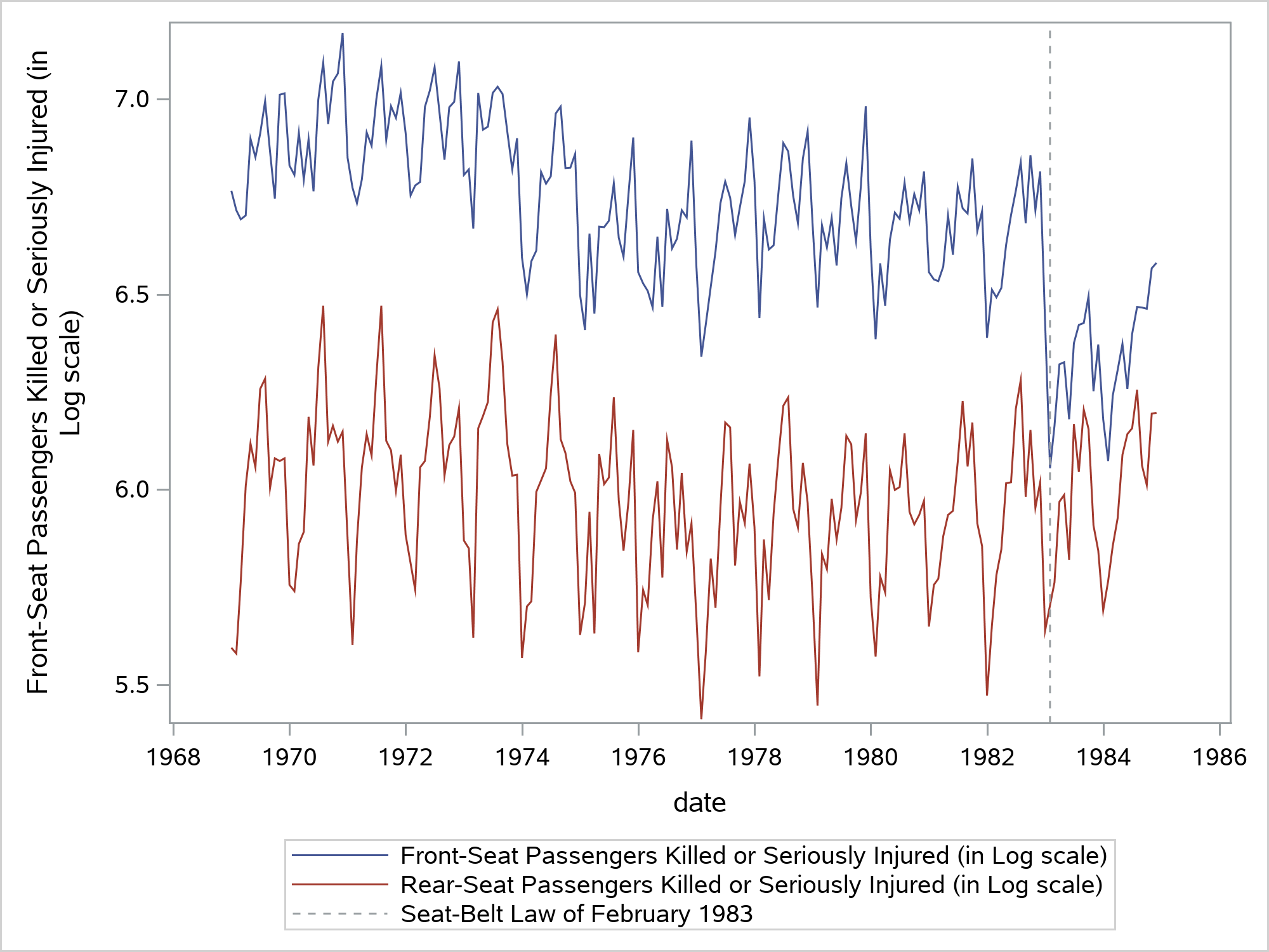
From the time series plots you can see that:
- F_KSI and R_KSI numbers don’t show a pronounced upward or downward trend but do show monthly seasonal variation
- These two series seem to move together, at least till February 1983. Starting in February 1983, the mean level of F_KSI appears to drop whereas the R_KSI pattern seems to remain unaffected.
The drop in the mean level of F_KSI is attributed to the enactment of the seat-belt law of February 1983. This law required the front seat passengers to wear seat belts. It didn’t apply to the rear seat passengers. These data have been analyzed by many researchers in the past.
Stability monitoring of monthly traffic accident numbers
In this section, we will see how you can perform a model-based stability monitoring of the bivariate series (F_KSI, R_KSI). We will use data from January 1969 to December 1981 as the initial portion of the series. This is used for fitting a suitable model and to create the score store. Note that the drop in the mean level of F_KSI, which happened in February 1983, is not part of this initial portion. We hope to detect this drop during the stability monitoring of this series, which begins from January 1982.
Denoting by Yt the bivariate series (F_KSI, R_KSI), and by Xt \(\beta\) the regression effects of logKM and logPrice, the model Yt = Xt \(\beta\) + \(\mu\)t + \(\gamma\)t + \(\epsilon\)t has been shown to be a reasonable model for this initial portion of the series. Here \(\mu\)t denotes the mean level, \(\gamma\)t denotes the monthly seasonal component, and \(\epsilon\)t denotes the noise component (all the terms in the model are bivariate). The data table mycas.train contains the initial portion of the series. The following statements fit this model and create the score store, mycas.inscore:
proc cssm data=mycas.train; id date interval=month; state wn(2) type=WN cov(g); comp wn1 = wn[1]; comp wn2 = wn[2]; state meanLevel(2) type=RW cov(rank=1) checkbreak; comp f_KSI_Level = meanLevel[1]; comp r_KSI_Level = meanLevel[2]; state season(2) type=season(length=12); comp f_KSI_season = season[1]; comp r_KSI_season = season[2]; model f_KSI = f_KSI_Level logKM logPrice f_KSI_season wn1; model r_KSI = r_KSI_Level logKM logPrice r_KSI_season wn2; output break(alpha=0.01) ao(alpha=0.01); score out(8)=mycas.inscore; run; |
The score store, mycas.inscore, saves the following information:
- Model specification and parameter estimates
- This also includes the user-specified outlier and structural break detection options such as the CHECKBREAK option in the specification of the bivariate mean level, and the significance levels of the structural break and outlier detection tests (0.01 for both types of tests in this case).
- Estimate of the latent state vector (and its covariance), which serves as a bridge between the past and the future.
- The last 8 rows, from May to December of 1981, of the input data table mycas.train. This is because we used the OUT(k)= form of the OUT option in the SCORE statement. This user-supplied, 8-observation window is used during the stability monitoring.
With the saved information in the score store, mycas.inscore, the model specification, or the historical data (mycas.train) are no longer needed to perform the stability monitoring of the future observations. During the stability monitoring, new observations arrive one at a time. This new observation gets read into a one-row table, mycas.nextObs, which, in turn, gets scored:
proc cssm data=mycas.nextObs; score in=mycas.inscore out=mycas.outscore; run; |
This simple scoring step accomplishes two key operations:
- The 9 observations, which are formed by joining the new observation with the 8-observation sliding window of the preceding observations that is stored in mycas.inscore, are scanned for any structural breaks or additive outliers
- An updated score store, mycas.outscore, is created by utilizing the new observation
After each scoring step, the two score stores (mycas.inscore and mycas.outscore) are swapped so the new observation always gets scored using the latest information. See SAS Help Center: Scoring: Monitoring Streaming Data for a complete code illustration of these steps. In our example, stability monitoring starts in January 1982. The main findings of the monitoring process are as follows:
- No breaks in the mean pattern or additive outliers are found between January 1982 and January 1983
- Starting with February 1983, for the next several months, the structural break/outlier detection tests flag February 1983 as an unusual month for two reasons:
- Drop in the mean level of F_KSI, which is called a level shift (LS)
- The unusually low value of F_KSI, which is called an additive outlier (AO)
The following table shows a summary of this monitoring process:
- New_Obs column shows the month of the observation that was scored
- AO_Z and LS_Z columns show the Z-statistics for these AO and LS tests, respectively
| New_Obs | AO_Z | LS_Z |
| FEB83 | -7.13 | -7.13 |
| MAR83 | -6.57 | -8.83 |
| APR83 | -6.43 | -9.19 |
| MAY83 | -6.22 | -9.89 |
| JUN83 | -5.97 | -10.63 |
| JUL83 | -5.84 | -11.41 |
Clearly, the Z-statistics for both AO and LS are highly significant in all the months between February and July. However, the significance of LS increases steadily whereas the significance of AO decreases steadily. This strongly points to February 1983 being a level shift for F_KSI, rather than a one-off value.
Usually when a structural break, such as a shift in the mean level, is detected, the monitoring is suspended. Before the monitoring can resume, you must update the model to account for the break. Or the cause for the break must be addressed by making appropriate changes to the mechanics of the observation process. In this traffic monitoring case, the monitoring can resume after the model is updated to account for the effect of the seat-belt law. In this example, a break in mean level was detected. You can use both PROC CSSM (and PROC SSM) to detect more general types of breaks.
Conclusion
Streaming data and their monitoring, usually without explicit human intervention, are happening everywhere. SAS Viya provides excellent tools for dealing with such data (for example, SAS Analytics for IoT). The new scoring capability in PROC CSSM (or the underlying CAS actions ssmFit and ssmScore) is designed to neatly fit in such applications.
LEARN MORE | SAS Viya LEARN MORE | SAS Econometrics


1 Comment
Cool stuff Rajesh, can't wait to see the %macro STREAM in action! Thank you very much for the interesting blog! 🙂