Recently, we’ve released a new feature in ASTORE: score with multiple analytic stores. In the process, we may create multiple analytic stores with dependencies among them (the output of some analytic stores is an input to others). This feature streamlines the scoring process of multiple analytic stores. It enables the scoring of one observation at a time with each analytic store to produce the desired final output. It eliminates the need for saving to intermediate files. We will use the Titanic data set as an example to show the streamlined scoring process of ASTORE and compare it with the Open Neural Network Exchange (ONNX) model scoring process.

Introduction

ASTORE is a system that allows a user to save the state from a predictive analytic procedure/action and to score the new data with the saved state. The state from a predictive analytic procedure/action is created using the results from the model development. It is usually a binary file, which is called an analytic store. In model deployment, the analytic store is restored to the state of the predictive model for scoring new data.

Before a model is built, we typically need to preprocess the data. For example, the input data may have missing values, and so we may want to impute the missing values with different methods. The dataPreprocess action set provides several actions for this purpose. These actions can also produce an analytic store. Together with the analytic stores for the predictive models, we’ll need to score the new data with multiple stores.

Below, Patrick Koch, my co-author, and I illustrate how ASTORE streamlines the scoring process of multiple stores.

The Titanic example

We’ll use the Titanic data set as an example to build models and demonstrate the capabilities of the new feature in ASTORE. The target variable is survival, which indicates whether or not the passenger survived. As in the example, we’ll use five predictor variables: three categorical (embarked, sex, pclass) and two numeric (age, fare). We first partition the input data into train and test by using the Simple Random Sampling (srs) action.

Since there are missing values in the predictor variables, we impute them before building the models. For categorical variables, we use the mode; for numeric variables, we use the median. We also standardize the numerical variables and use the one-hot encoding method for the categorical variables.

The SAS code for partitioning the data and the data preprocessing is shown below.

  /* the Titanic data set is available at 
   https://raw.githubusercontent.com/amueller/scipy-2017-sklearn/091d371/notebooks/datasets/titanic3.csv
   */
   proc casutil;
           load file="titanic3.csv" casout="titanic3" ;	*load the data;
   run;
 
   %let in_numeric_features = %str('age' 'fare');
   %let in_categorical_features = %str('embarked' 'sex' 'pclass');
   %let target = 'survived';
   %let in_all_features = %str(&in_numeric_features  &in_categorical_features &target);
 
 
   proc cas;
     loadactionset "sampling"; run;
     loadactionset "dataPreprocess"; run;
     loadactionset "regression"; run;
 
     /*partition the data to train and test with a partition indicator*/
     action sampling.srs /
       table="titanic3"
       samppct=20 seed=17 partInd=true
       output={casout={name='titanic' replace=true} copyvars={&in_all_features}};
     run;
 
 
     /*call the transform action for the preprocessing on the train data*/
     action dataPreprocess.transform /
       table={name='titanic', where='_PartInd_=0'},
       pipelines = {
                     {inputs = {&in_numeric_features},
                      impute={method='median'},                      /*impute the numeric features by median*/
                      function={method='standardize', args={location='mean', scale='std'}}                /*standardize*/
                     },
                     {inputs = {&in_categorical_features},
                      impute={method='mode'},                            /*impute the categorical features by mode*/
                      cattrans={method='onehot'}                         /*encode with the onehot method*/
                     }
                   },
       outVarsNameGlobalPrefix = 't',                   /*common prefix for the transformed variables*/
       saveState = {name='transstore', replace=True};     /*save the state to an analytic store*/
     run;
 
 
    /*call scoring to get the transformed train data*/
     action aStore.score/
       rstore='transstore',
       table={name='titanic', where='_PartInd_=0'},
       copyvars= (&target),
       casout={name='trans_out',replace=True};
     run;

After preprocessing the data, we build the logistic model as follows:

     /*call the logistic action to build a logistic model and save to an analytic store*/
     action regression.logistic/
       table='trans_out',
       classvars={'t_embarked', 't_sex', 't_pclass'},
       model={depvar=&target,
              effects={'t_embarked', 't_sex', 't_pclass', 't_age', 't_fare' }},
       store={name='logstore', replace=True};
     run;

Score with multiple analytic stores

Now we have two analytic stores: one named transstore from the transform action, the other named logstore from the logistic action. To score the test data, we just specify the two stores in the score action as follows:

   *score the test data with multiple analytic stores;
     action aStore.score/
       multiplerstores={{name='logstore'}, {name='transstore'}},
       table={name='titanic', where='_PartInd_=1'},
       casout={name='test_out',replace=True};
     run;

For the equivalent code in SAS procs, see SAS Viya Machine Learning on GitHub.

When specifying multiple analytic stores in the score action, their order does not matter. ASTORE will automatically determine the dependence among the stores based on the input and output variables of each store. If an output variable of store A is an input variable of store B, then store B depends on store A. From the stores and the dependencies among them, ASTORE creates a directed graph with the nodes being the vertices and edges being the dependences. The graph is used to decide the order of scoring with these analytic stores.

For the above two stores, the logistic store (logstore) depends on the transform store (transstore) because the output variables of the transform store are the input of the logistic store. For each observation in the test data, it will first be scored with the transform store. Then the output of the transform store is fed into the logistic store as input. The output of the logic store is the final output of the scoring.   The flow of the scoring process is shown in Figure 1.

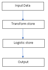
Figure 1: ASTORE flow

The scoring process works similarly if there are more than two analytic stores. First, the dependence between any pair of stores is determined based on their input and output variables. Then a directed graph is built with each analytic store being a vertex and the dependence between two stores being edges. The graph is used to decide the order of scoring. As long as there are no cycles in the graph, the scoring is done in the order of the dependencies.

Without such a streamlining process, we would have to score the entire data with each analytic store manually. For the Titanic example, we could score the test data first with the transform store and save the results to a temporary table. Then we feed the temporary table to the logistic store for scoring to get the final output. This manual process gets worse with more analytic stores.

As shown in [1], we can also apply similar data preprocessing the Titanic data and then build a logistic model with scikit-learn [2]. The logistic model together with the data preprocessing steps can be saved to an Open Neural Network Exchange (ONNX) file. The ONNX file consists of standard operators, which are connected by data (usually tensors). The graph corresponding to the logistic model on the Titanic data is shown in Figure 2.

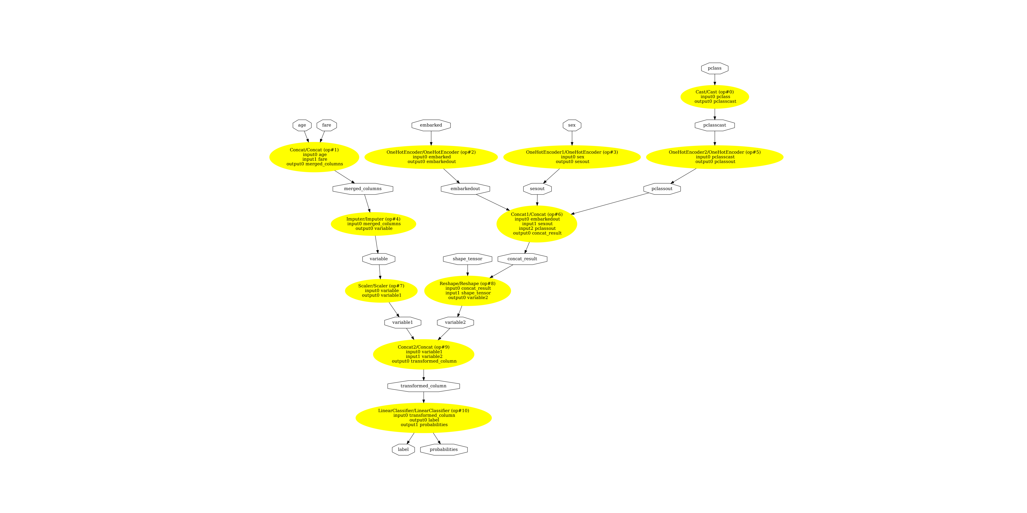
Figure 2: ONNX pipeline

An ONNX file can be used to score new data through an ONNX runtime as shown in [1]. The scoring is done at the observation level, which is similar to ASTORE. However, the pipeline looks more complex than the ASTORE one in Figure 1. With ASTORE, we only need two analytic stores for this example, while the ONNX standard operators are defined at a lower granular level, which results in a complex pipeline.

Summary

We have used the Titanic data set as an example to demonstrate the capabilities of ASTORE. This post has shown that scoring with multiple analytic stores is streamlined at the observation level through a simple flow.  Also indicated is that similar functionalities can be done through ONNX, which however has a complex pipeline.

References

[1] http://onnx.ai/sklearn-onnx/auto_examples/plot_complex_pipeline.html#sphx-glr-auto-examples-plot-complex-pipeline-py

[2] https://scikit-learn.org/stable/