This is the third and final installment in a series of posts explaining  complex models in SAS® Viya®. My SAS colleague Funda Gunes is my co-author.  

In the preceding two posts, we looked at issues around the interpretability of modern black-box machine-learning models and introduced techniques available in SAS® Model Studio within SAS® Visual Data Mining and Machine Learning. Now we turn our attention to programmatic interpretability using SAS® Cloud Analytic Services directly.

Introduction to the explainModel action set

The actions in the explainModel action set can be used to explain a model whose score code is saved in SAS DATA Step code or a SAS analytic store. The action set includes three actions:

• The partialDependence action calculates partial dependence (PD) and individual conditional expectation (ICE), which explain model behaviors on a variable-by-variable basis.
• The linearExplainer action also provides both local and global explanations. The local explanations (Shapley value estimates and LIME values) provide information about variable influence and local model behavior for an individual observation, and the global explanations (global regression) shed light on the overall model behavior by fitting a global surrogate regression model. The Shapley value estimator in the linearExplainer action uses the Kernel SHAP method.
• The shapleyExplainer action is a specialized Shapley value explainer that provides scalable and accurate Shapley value estimates. The Shapley values reflect the contribution of each variable toward the final prediction for an individual observation. The shapleyExplainer action uses the HyperSHAP method to calculate the Shapley values.

For implementation details about these techniques and user options, see the chapter “Explain Model Action Set” in SAS Visual Data Mining and Machine Learning 8.5: Programming Guide.

Case study: detecting breast cancer with machine learning

Diagnosing illness is a frequent and difficult task for doctors in the health-care industry. An incorrect diagnosis can mean severe consequences. To help doctors, many studies employ machine learning by training a model on historical clinical cases. Unfortunately, lacking adequate interpretations, many of the most complex machine learning models cannot participate in some diagnostic procedures.

This section uses a health-care application to demonstrate how to access interpretability through a programmatic interface. The full SAS Viya code for this example can be found on github. We will uses the interpretability actions available in SAS Viya to train a model that predicts the malignancy of potential breast cancer biopsies and to explain the predictions of this model.

Data for this section is from the University of Wisconsin Hospitals in Madison, WI, from Dr. William H. Wolberg, as described by Mangasarian and Wolberg (1990). The data contain nine observed quantities that are calculated by a physician upon the collection of a fine needle aspirate (FNA) from a potentially malignant area in a patient and are labeled according to their malignancy.

The data contains nine input variables and a target variable. The input variables are clump thickness, uniformity of cell size, uniformity of cell shape, marginal adhesion, single epithelial cell size, bare nuclei, bland chromatin, normal nucleoli, and mitoses. Each of these variables ranges from 1 to 10, with larger numbers generally indicating a greater likelihood of malignancy according to the examining physician. The target variable indicates whether the region was malignant or benign. Not one of these input variables by itself is enough to determine whether the region is malignant, so they must be aggregated in some way. A random forest model is trained to predict sample malignancy from these variables.

The data contains 699 observations. The bare nuclei variable contains a few instances of missing data, which were imputed to have value 0. The data was partitioned into a training set (70%) and a test set (30%). The following code trains a random forest model on the training data by using the decisionTree action set in SAS Visual Data Mining and Machine Learning:

proc cas; 
 
    inputs = &inputs; 
    decisionTree.forestTrain result = forest_res / 
        table = "BREAST_CANCER_TRAIN" 
        target = "class" 
        inputs = inputs 
        oob = True 
        nTree = 500 
        maxLevel = 12 
        prune = True 
        seed = 1234 
        varImp = True 
        casOut = {name = "FOREST_MODEL_TABLE", 
                  replace = True} 
        savestate = {name = "FOREST_MODEL", 
                     replace = True}; 
    run; 
 
quit;

The macro variable &inputs defines a list that contains the names of the input variables (except the ID variable). Following this training, a cutoff of 0.4 was selected to optimize the model’s misclassification rate on the training set. This cutoff was then used to assess the model on the test set, which achieved a misclassification rate of 2.91%. This accuracy is competitive with other black-box models that are trained and published on the same data.

Although the predictive accuracy is good, the forest model remains difficult to interpret because of its complexity. This complexity can render the model entirely useless in clinical settings, where interpretability is paramount for a patient’s well-being and the physician’s confidence.

Variable importance

Table 1 contains the model-specific variable importance of the input variables as calculated by the forestTrain action.

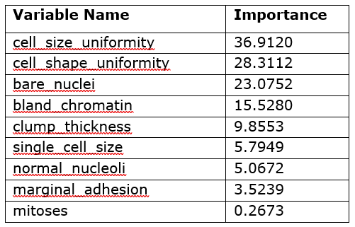
Table 1 shows that the five most important variables for the model’s predictions are the uniformity of cell size and shape, bare nuclei, bland chromatin, and clump thickness. As you can see, this table does not tell you the direct effect of these variables in the model; it only says which variables were important in the model’s construction. However, you can use this information to decide which variables to investigate further through other interpretability techniques such as PD and ICE plots.

The preceding information establishes that the forest model is highly predictive on unseen data and that not all the input variables are equally important. One remaining question is how each of the input variables affects the prediction of the model. The partial dependence plots for a particular variable illustrate how the model’s predictions change when that variable’s value fluctuates with all other variables being held constant.

The following CAS action call requests the partial dependence plot for the most important variable (cell size uniformity) of the variable importance table:

proc cas; 
 
    /* Inputs and Nominals macro -> CASL Var */ 
    inputs = &inputs; 
 
    /* Action Call */ 
    explainModel.partialDependence result = pd_res / 
        table = "BREAST_CANCER" 
        inputs = inputs 
        modelTable = "&model" 
        modelTableType = "ASTORE" 
        predictedTarget = "&pred_target" 
        analysisVariable = {name  = "&var_name",  
                            nBins = 50} 
        iceTable = {casout = {name = "ICE_TABLE", replace = True}, 
                    copyVars = "ALL"} 
        seed = 1234;
    run; 
 
    /* Save PD Results */ 
    saveresult pd_res["PartialDependence"] dataset = PD_RES; 
    run; 
 
quit;

Again, the &inputs macro variable is used to specify the list of input variables to the partialDependence action. The modelTable, modelTableType, and predictedTarget parameters specify the model being explained and its expected output column. The table and iceTable parameters indicate which data sets to use for the PD calculation and for storing replicated observations, respectively. The variable being explained is specified in the analysisVariable parameter, which contains other subparameters for slightly altering the produced PD calculation. For more information, see the chapter “Explain Model Action Set” in SAS Visual Data Mining and Machine Learning 8.5: Programming Guide.

 Figure 1 shows the partial dependence of the forest’s predictions with respect to the cell size uniformity variable.

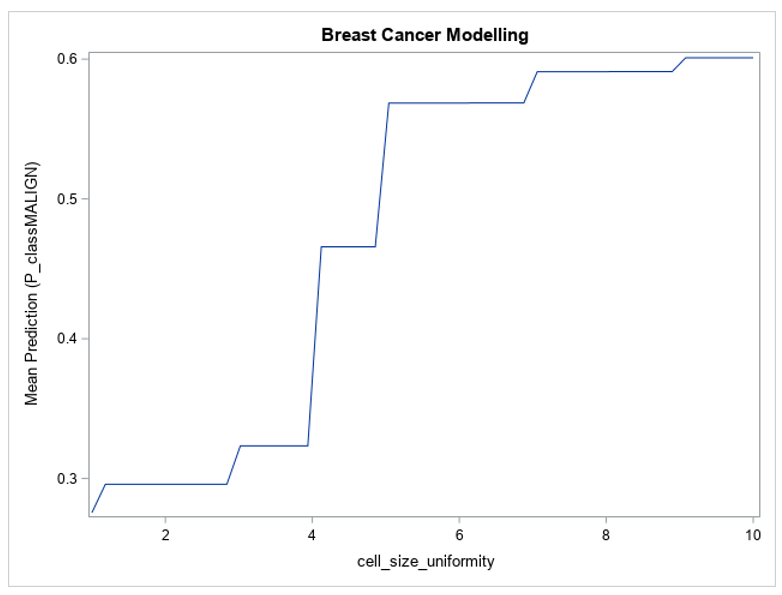
Figure 1 shows that the model’s predictions change greatly between the extremes of the cell size uniformity variable — for lower values of cell size uniformity, the model’s average prediction is lower than 0.3, and for larger values it reaches 0.6. The value of this variable in the input data can have a large effect on the prediction from the model, which is why its variable importance metric is so high. Figure 1 also shows that the model’s prediction with respect to cell size uniformity is monotonic, always increasing as the variable’s value increases, which is as expected based on the description of the data. This plot builds trust in the model by demonstrating that it is not behaving in an unexpected way.

Typically, the partial dependencies of variables are shown on individual plots. However, since all the input variables in this problem lie on the same scale and have similar impact on the target (larger values indicate increased chance of malignancy), the partial dependencies with respect to each variable can be overlaid as shown in Figure 2.

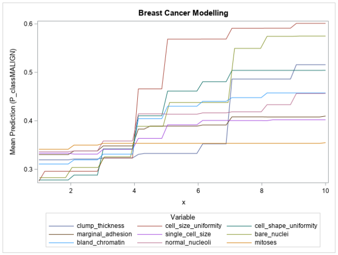
Figure 2 shows that the input variables are being used exactly as defined by the data description; the mean prediction of the model increases as the value of each of the input variables increases. Also depicted is the relative influence of each variable on the model’s prediction, with cell size uniformity, cell shape uniformity, bare nuclei, clump thickness, and bland chromatin all showing a large range in their mean predictions. These large ranges correspond to their high variable importance values and build further trust in the model. The mitoses variable’s partial dependence plot is almost perfectly flat, which would indicate that the variable contributes almost nothing to the prediction of the model.

LIME and HyperSHAP

The partial dependence plots are useful for understanding the effect of input variables on all observations. Sometimes, however, the role of a variable for an individual observation can be rather different from the role of that variable for the overall population. For example, for a particular patient, it would be useful to be able to determine which variables in an observation contribute most to the prediction of malignancy so that the patient could be further convinced of the need of a biopsy, a costly but necessary follow-up procedure. A reason such as “The thickness of the clumps in the FNA procedure lead us to believe that we should proceed with a biopsy” is more convincing to a patient than just saying “Looking at your FNA, we think we should proceed with a biopsy.” Explanations like these can be generated by using LIME and Shapley value methods.

The following code is used within a SAS macro to compute LIME coefficients:

explainModel.linearExplainer result = lex_res / 
    table = "BREAST_CANCER_TRAIN" 
    query = {name = "BREAST_CANCER_TRAIN",  
             where = "sample_id = &observation;"} 
    inputs = inputs 
    modelTable = "FOREST_MODEL" 
    modelTableType = "ASTORE" 
    predictedTarget = "P_classMALIGN" 
    preset = "LIME" 
    explainer = {standardizeEstimates = "INTERVALS", 
                 maxEffects = &num_vars+1} 
    seed = 1234; 
run;

In the code, the preset parameter is used to select the LIME method for generating explanations. The table, modelTable, modelTableType, and predictedTarget parameters are used in the same way as in the previous partialDependence action call; they specify the data and model to use. The &observation macro variable specifies which observation’s prediction is being explained, and the &num_vars macro variable species how many input variables are being reported by LIME. The standardizeEstimates parameter is set to INTERVALS, which tells the action to standardize the least squares estimates of the LIME coefficients so that their magnitudes can be compared.

The following code is used to compute the Shapley values for explaining an individual prediction:

explainModel.shapleyExplainer result = shx_res / 
    table = "BREAST_CANCER_TRAIN" 
    query = {name = "BREAST_CANCER_TRAIN",  
             where = "sample_id = &observation;"} 
    inputs = inputs 
    modelTable = "FOREST_MODEL" 
    modelTableType = "ASTORE" 
    predictedTarget = "P_classMALIGN"; 
run;

As in the linearExplainer action call, the &observation macro variable in the shapleyExplainer call is used to specify the observation to be explained. The shapleyExplainer action call reuses all previous parameters: table, query, inputs, modelTable, modelTableType, and predictedTarget. The values of the input variables for the specified observation are shown in Table 2. This observation was determined by the physician to be malignant. The input variables in this observation are large, which would correspond to a high likelihood of malignancy according to the attending physician. The forest model produces a predicted probability of 100% that this observation is malignant.

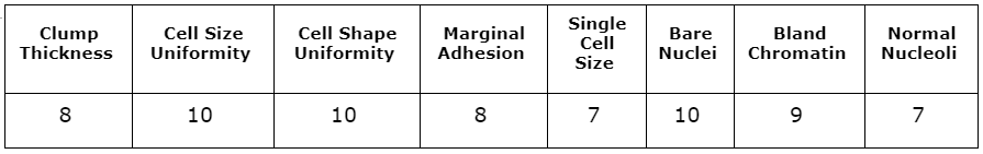
Figure 3 shows the LIME coefficients for explaining the forest model for the observation that is shown in Table 2.

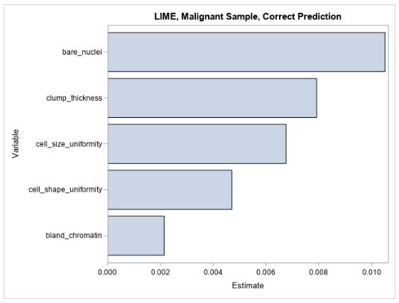
The LIME values for the observation are all positive, indicating that the model’s prediction increases as each variable value increases in the local region around this observation. This local explanation agrees with the global explanation that comes from the partial dependence plots, where the mean prediction increases along with each input variable.

Figure 4 shows the five largest Shapley values for explaining the prediction for the same observation that is shown in Table 2.

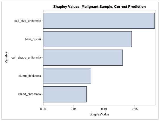
The Shapley values for this observation are all positive, indicating that the values of the input variables to the model in this observation increase the model’s prediction relative to other observations in the training data. This makes sense because the input variables in this observation are all high, taking values between 7 and 10, which would all indicate high likelihood for malignancy, and thus contribute positively to the model’s prediction. You can see that LIME and Shapley explanations mostly agree for explaining the pre-trained forest model’s prediction for this observation.

Table 3 shows another sample from the data for which the model produced an incorrect prediction. Although the sample did prove to be malignant, the model predicts a likelihood of malignancy of 0.14, which is a large deviation from the truth. Most of the input variables in this observation take low values, meaning the investigating physician did not think any variable indicated a strong likelihood of malignancy. The LIME and Shapley values might provide insight into why the model produces this prediction.

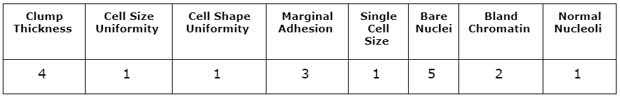
Figure 5 shows the LIME coefficients for explaining the forest model’s false prediction.

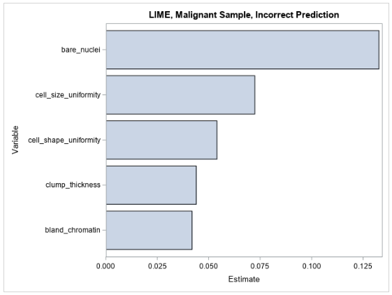
The LIME coefficients offer little insight beyond what is already understood about the model—that its prediction increases with respect to each increasing input variable. Many of the variables’ values are small in this observation, and it would therefore be expected that the model’s prediction would also be small.

Figure 6 shows the Shapley values for the same observation that is shown in Table 3.

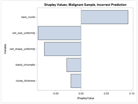
The Shapley values for the observation are more meaningful in the context of the incorrect prediction. It appears that the only variable that contributes positively to the prediction of malignancy is the bare nuclei variable (which takes an intermediate value of 5) and that all other input values cause the model’s prediction to decrease with respect to the other observations. It seems that the model is split in determining whether this observation is malignant. This can be caused by the model giving too much weight to some variables or there not being enough information in the input data to model this observation. Ultimately these results can identify a weakness in the modeling process or might indicate that this particular instance is really hard to diagnose on the basis of the available input variables. This information can be used to inform further data collection, feature engineering, and model tuning.

Refining the model

Model interpretability does not necessarily need to be confined to the end of a modeling process. Occasionally, the interpretability results can reveal information that leads to new feature engineering ideas or reveals that certain input variables are useless to the models and only contribute to the curse of dimensionality. For this data set, the partial dependency of the input variables increases monotonically. The simple nature of the relationship between the input variables and the model’s prediction might lead you to think that a simpler model will perform just as well as the forest model for this problem. Furthermore, the mitoses variable seems to be effectively unused by the model according to both the variable importance table and the partial dependence plots, which means it can likely be dropped entirely from the input data.

With the preceding information in mind, a logistic regression model is trained on the same data, dropping the mitoses input. Backwards selection is done using the logistic action in the regression action set. Only the clump thickness, cell size uniformity, and bare nuclei variables remain after selection. Based on the training data, a cutoff of 0.19 is selected, which yields a misclassification rate of 4.37% on the test set, a mere 1.46% decrease in accuracy from the forest model. Figure 7 shows the partial dependence of each input variable with respect to the mean prediction from the logistic model.

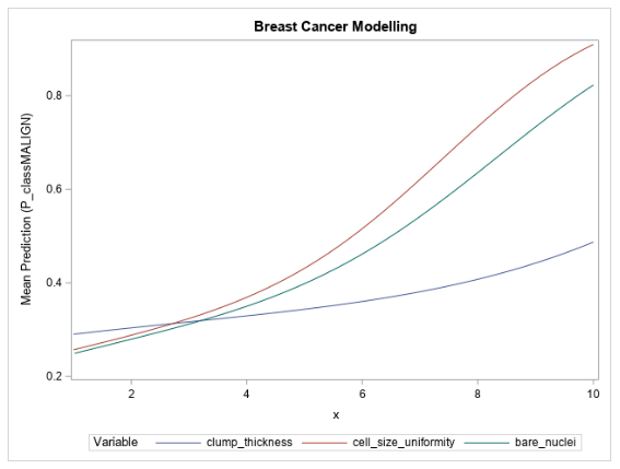
The partial dependence curves of the input variables for the logistic regression model show a similar relationship to what they show in the forest model, with the mean prediction increasing as the variable values increase. However, as expected, the logistic curves are much smoother than those of the forest model.

Now you have two models of comparable accuracy, each with its drawbacks. The forest model demonstrates a higher accuracy than the regression model, but it is natively uninterpretable. The logistic regression enables you to directly use the regression coefficients to understand the model, but it has a slightly lower accuracy. Ultimately the best model to use is the one that maximizes prediction accuracy while meeting the necessary interpretability standard. If using the LIME, Shapley, and partial dependence values for interpretations provides meaningful explanations given the modeling context, then the forest model is better. If not, then the logistic regression should be chosen. Since this model will ultimately be consumed by a clinician who has worked closely with the patient and directly developed the input features, the forest model is likely a better choice, because the clinician is there to safeguard against model inaccuracies.