If you spend any time working with maps and spatial data, having a fundamental understanding of coordinate systems and map projections becomes necessary. It’s the foundation of how spatial data and maps work. These areas invariably evoke trepidation and some angst, even in the most seasoned map professional. And rightfully so, it can get complicated quickly. Fortunately, most of those worries can be set aside when creating maps with SAS Visual Analytics, without requiring a degree in Geodesy.
Visual Analytics includes several different coordinate system definitions configured out-of-the-box. Like the Predefined geography types (see Fundamental of SAS Visual Analytics geo maps), they are selected from a drop-down list during the geography variable setup. With the details handled by VA, all you need to know is what coordinate space your data uses and select the appropriate one.
The four Coordinate spaces included with VA are:
- World Geodetic System (WGS84)
Area of coverage: World. Used by GPS navigation systems and NATO military geodetic surveying. This is the VA default and should work in most situations. - Web Mercator
Area of coverage: World. Format used by Google maps, OpenStreetMap, Bing maps and other web map providers. - British National Grid (OSGB36)
Area of coverage: United Kingdom – Great Britain, Isle of Man - Singapore Transverse Mercator (SVY21)
Area of coverage: Singapore onshore/offshore
But what if your data does not use one of these? For those situations, VA also supports custom coordinate spaces. With this option, you can specify the definition of your desired coordinate space using industry standard formats for EPSG codes or Proj4 strings. Before we get into the details of how to use custom coordinate spaces in VA, let’s take a step back and review the basics of coordinate spaces and projections.
Background
A coordinate space is simply a grid designed to cover a specific area of the Earth. Some have global coverage (WGS84, the default in VA) and others cover relatively small areas (SVY21/Singapore Transverse Mercator). Each coordinate space is defined by several parameters, including but not limited to:
- Center coordinates (origin)
- Coverage area (‘bounds’ or ‘extent’)
- Unit of measurement (feet or meters)
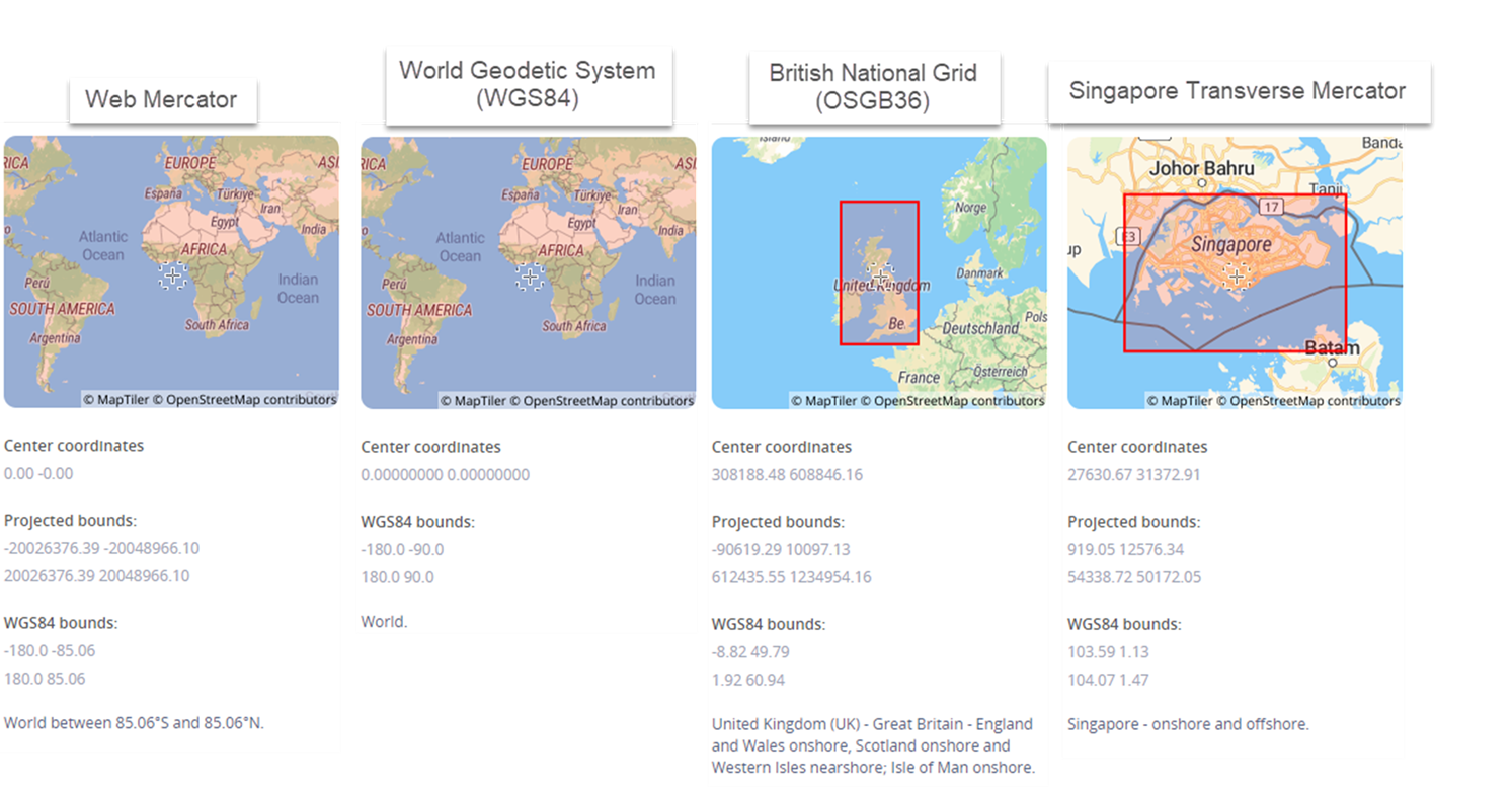
The image above compares the four coordinate space definitions included with VA. The two on the right, BNG and Singapore Transverse Mercator, have a limited extent. A red rectangle outlines the area of coverage for each region. The two on the left, WGS84 and Mercator, are both world maps. At first glance, they may appear to have the same coverage area, but they are not interchangeable. The origin for both is located at the intersection of the Equator and the Prime Meridian. However, the similarities end there. Notice the extent for WGS84 covers the entire latitude range, from -90 to +90. Mercator on the other hand, covers from -85 to +85 latitude, so the first 5 degrees from each Pole are not included. Another difference is the unit of measurement. WGS84 is measured in un-projected degrees, which is indicative of a spherical Geographic Coordinate System (GCS). Mercator uses meters, which implies a Projected Coordinate System (PCS) used for a flat surface, ie. a screen or paper.
The projection itself is a complex mathematical operation that transforms the spherical surface of the GCS into the flat surface of the PCS. This transformation introduces distortion in one or more qualities of the map: shape, area, direction, or distance. The process of map projection is often compared to peeling an orange. Removing the peel and placing it on a flat surface will cause parts of it to stretch, tear or separate as it flattens. The same thing happens to a map when it is projected.
A flat map will always have some degree of distortion. The type and amount of distortion depends on the projection used. A projection should be selected to minimize the distortion in the areas most important to the map. For example, are you creating a navigation map where direction is critical? How about a World map to compare land mass of various countries? Or maybe a local map of Municipality services where all factors are equally important? These decisions are important if you are collecting and creating your data set from the field. But, if you are using existing data sets, chances are that decision has already been made for you. It then becomes a task of understanding what coordinate system was selected and how to use it within VA.
Using a Custom Coordinate Space in VA
When using VA’s custom coordinate space option, it is critical the geography variable and the data set use the same coordinate space. This tells VA how to align the grid used by the data with the grid used by the underlying map. If they align, the data will be placed at the expected location. If they don’t align, the data will appear in the wrong location or may not be displayed at all.
To illustrate the process of using a custom coordinate space in VA, we will be creating a custom region map of the Oklahoma City School Districts. The data can be found on the Oklahoma City Open Data Portal. We will use the Esri shapefile format. As you may recall from a previous blog post, Creating custom region maps with SAS Visual Analytics, the first step is to import the Esri shapefile data into a SAS dataset.
Once the shapefile has been successfully imported into SAS, we then must determine the coordinate system of the data. While WGS84 is common and will work in many situations, it should not be assumed. The first place to look is at the source, the data provider. Many Open Data portals will have the coordinate system listed along with the metadata and description of the data set. But when using an Esri shapefile, there is an easier way to find what we need.
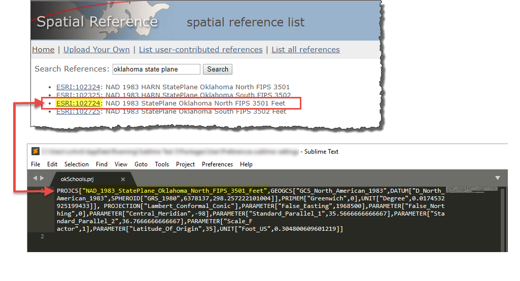
Locate the directory where you unzipped the original shapefile. Inside of that directory is a file with a .prj extension. This file defines the projection and coordinate system used by the shapefile. Below are the contents of our .prj file with the first parameter highlighted. We are only interested in this value. Here, you can see the data has been defined in the Oklahoma State Plane coordinate system -- not in VA’s default WGS84. So, we must use a custom coordinate system when defining the geography variable.
PROJCS["NAD_1983_StatePlane_Oklahoma_North_FIPS_3501_Feet",GEOGCS["GCS_North_American_1983",DATUM["D_North_American_1983",SPHEROID["GRS_1980",6378137,298.257222101004]],PRIMEM["Greenwich",0],UNIT["Degree",0.0174532925199433]], PROJECTION["Lambert_Conformal_Conic"],PARAMETER["False_Easting",1968500],PARAMETER["False_Northing",0],PARAMETER["Central_Meridian",-98],PARAMETER["Standard_Parallel_1",35.5666666666667],PARAMETER["Standard_Parallel_2",36.7666666666667],PARAMETER["Scale_Factor",1],PARAMETER["Latitude_Of_Origin",35],UNIT["Foot_US",0.304800609601219]]
Next, we need to look up the Oklahoma State Plane coordinate system to find a definition VA understands. From the main page of the SpatialReference.org website, type ‘Oklahoma State Plane’ into the search box. Four results are returned. Compare the results with the string highlighted above. You can see the third option is what we are looking for: NAD 1983 StatePlane Oklahoma North FIPS 3501 Feet.
To get the definitions we need for VA, click the third link for the option NAD 1983 StatePlane Oklahoma North FIPS 3501 Feet. Here you will see a grey box with a bulleted list of links. Each of these links represent a definition for the Oklahoma StatePlane coordinate space.
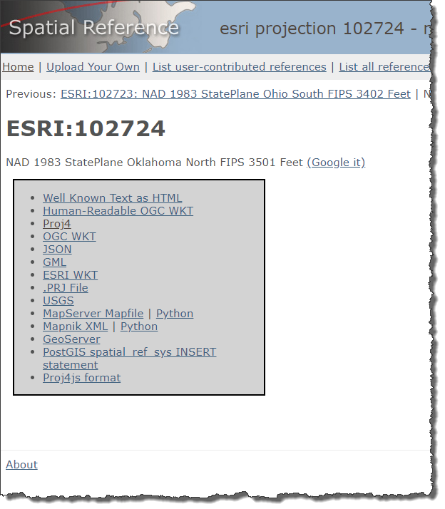
Visual Analytics supports two of the listed formats, EPSG and Proj4. EPSG stands for European Petroleum Survey Group, an organization that publishes a database of coordinate system and projection information. The syntax of this format is epsg:<number> or esri:<number>, where <number> is a 4-6 digit for the desired coordinate system. In our cases, the format we need is the title of the page:
ESRI:102724
The second format supported by VA is Proj4, the third link in the image above. This format consists of a string of space-delimited name value pairs. The Oklahoma StatePlane proj4 definition we are interested in is:
+proj=lcc +lat_1=35.56666666666667 +lat_2=36.76666666666667 +lat_0=35 +lon_0=-98 +x_0=600000.0000000001 +y_0=0 +ellps=GRS80 +datum=NAD83 +to_meter=0.3048006096012192 +no_defs
Now we have identified the coordinate system used by our data set and looked up its definition, we are ready to configure VA to use it.
Using a Projected Coordinate System definition in VA
The following section assumes you are familiar with custom region maps and setting up a polygon provider. If not, see my previous post on that process, Creating custom region maps with SAS Visual Analytics. The first step in setting up a geography variable for a custom region map is to start with the polygon provider. At the bottom of the ‘Edit Polygon Provider’ window, there is an ‘Advanced’ section that is collapsed by default. Expand it to see the Coordinate Space option. By default, it is populated with the value EPSG:4326, which is the EPSG code for WGS84. Since our Oklahoma City School District code data does not use WGS84, we need to replace this value with the EPSG code that we looked up from SpatialReference.org (ESRI:102724).
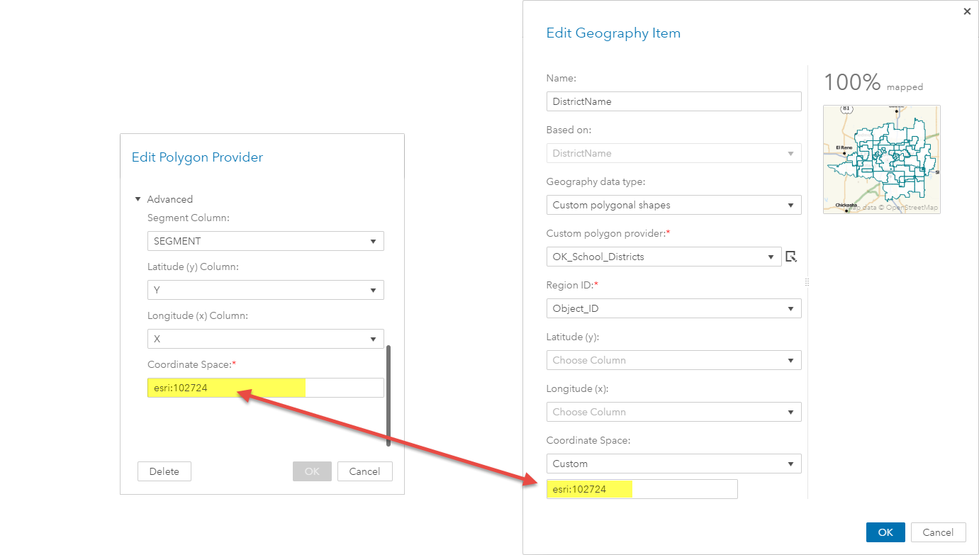
Next, we must make sure to configure the geography variable itself with the same coordinate space as the polygon provider. On the ‘Edit Geography Item’ window, the Coordinate Space option is the last item. Again, we must change this from the default WGS84 to ESRI:102724. From the dropdown list, select the option ‘Custom’. A new entry box appears where we can enter the custom coordinate space definition. If configured correctly, you should see your map in the preview thumbnail and a 100% mapped indicator.
Congratulations! The setup was successful. Now, simply click OK and drag the geography variable to the canvas. VA’s auto-map feature will recognize it and display the custom region map.
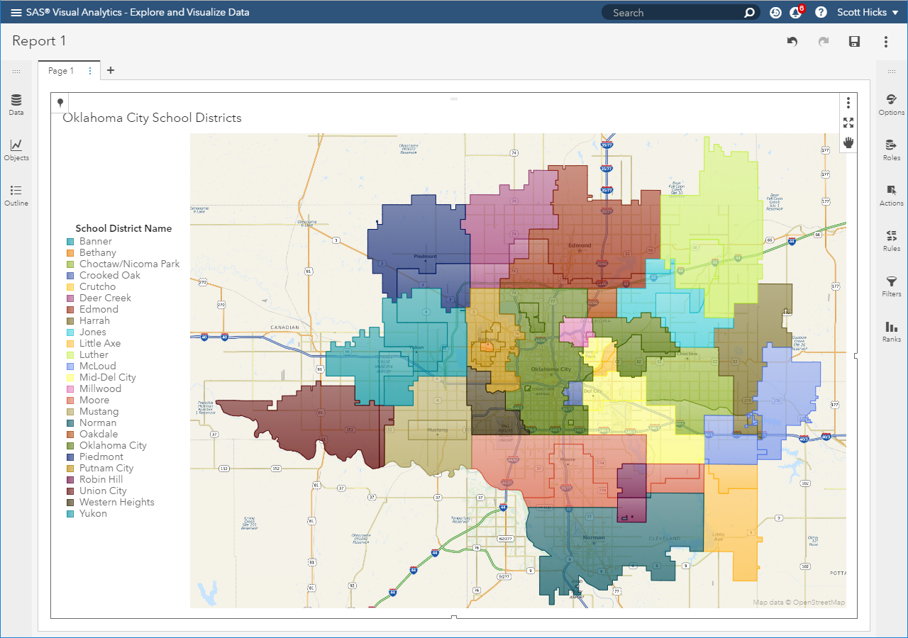
In this post, I showed how to identify the coordinate system of your Esri shapefile data, lookup its epsg and proj4 definitions, and configure VA to use it via the Custom Coordinate space option. While the focus was on a custom region map, the technique also applies to Custom Coordinate maps, minus the polygon provider setup. The support of custom coordinate spaces in VA allow the mapping of practically any spatial dataset, giving you a new level of power and flexibility in your mapping efforts.