Everyone’s excited about artificial intelligence. But most people, in most jobs, struggle to see the how AI can be used in the day-to-day work they do. This post, and others to come, are all about practical AI. We’ll dial the coolness factor down a notch, but we explore some real gains to be made with AI technology in solving business problems in different industries.

This post demonstrates a practical use of AI in banking. We’ll use machine learning, specifically neural networks, to enable on-demand portfolio valuation, stress testing, and risk metrics.

Background

I spend a lot of time talking with bankers about AI. It’s fun, but the conversation inevitably turns to concerns around leveraging AI models, which can have some transparency issues, in a highly-regulated and highly-scrutinized industry. It’s a valid concern. However, there are a lot of ways the technology can be used to help banks –even in regulated areas like risk –without disrupting production models and processes.

Banks often need to compute the value of their portfolios. This could be a trading portfolio or a loan portfolio. They compute the value of the portfolio based on the current market conditions, but also under stressed conditions or under a range of simulated market conditions. These valuations give an indication of the portfolio’s risk and can inform investment decisions. Bankers need to do these valuations quickly on-demand or in real-time so that they have this information at the time they need to make decisions.

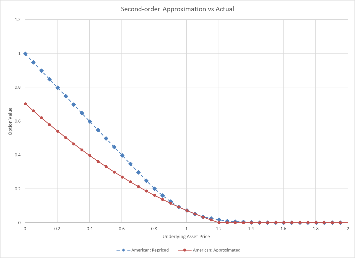
However, this isn’t always a fast process. Banks have a lot of instruments (trades, loans) in their portfolios and the functions used to revalue the instruments under the various market conditions can be complex. To address this, many banks will approximate the true value with a simpler function that runs very quickly. This is often done with first- or second-order Taylor series approximation (also called quadratic approximation or delta-gamma approximation) or via interpolation in a matrix of pre-computed values. Approximation is a great idea, but first- and second-order approximations can be terrible substitutes of the true function, especially in stress conditions. Interpolation can suffer the same draw-back in stress.

Improving approximation with machine learning

Machine learning is technology commonly used in AI. Machine learning is what enables computers to find relationships and patterns among data. Technically, traditional first- order and second-order approximation is a form of classical machine learning, such as linear regression. But in this post we’ll leverage more modern machine learning, like neural networks, to get a better fit with ease.

Neural networks can fit functions with remarkable accuracy. You can read about the universal approximation theorem for more about this. We won’t get into why this is true or how neural networks work, but the motivation for this exercise is to use this extra good-fitting neural network to improve our approximation.

Each instrument type in the portfolio will get its own neural network. For example, in a trading portfolio, our American options will have their own network and interest rate swaps, their own network.

The fitted neural networks have a small computational footprint so they’ll run very quickly, much faster than computing the true value of the instruments. Also, we should see accuracy comparable to having run the actual valuation methods.

The data, and lots of it

Neural networks require a lot of data to train the models well. The good thing is we have a lot of data in this case, and we can generate any data we need. We’ll train the network with values of the instruments for many different combinations of the market factors. For example, if we just look at the American put option, we’ll need values of that put option for various levels of moneyness, volatility, interest rate, and time to maturity.

Most banks already have their own pricing libraries to generate this data and they may already have much of it generated from risk simulations. If you don’t have a pricing library, you may work through this example using the Quantlib open source pricing library. That’s what I’ve done here.

Now, start small so you don’t waste time generating tons of data up front. Use relatively sparse data points on each of the market factors but be sure to cover the full range of values so that the model holds up under stress testing. If the model was only trained with interest rates of 3 -5 percent, it’s not going to do well if you stress interest rates to 10 percent. Value the instruments under each combination of values.

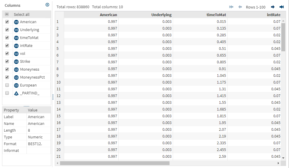
Here is my input table for an American put option. It’s about 800k rows. I’ve normalized my strike price, so I can use the same model on options of varying strike prices. I’ve added moneyness in addition to underlying.

The model

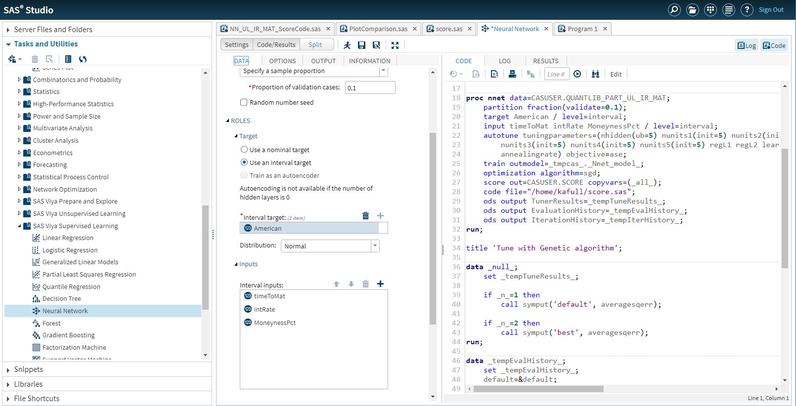
I use SAS Visual Data Mining and Machine Learning to fit the neural network to my pricing data. I can use either the visual interface or a programmatic interface. I’ll use SAS Studio and its programmatic interface to fit the model. The pre-defined neural network task in SAS Studio is a great place to start.

Before running the model, I do standardize my inputs further. Neural networks do best if you’ve adjusted the inputs to a similar range. I enable hyper-parameter auto-tuning so that SAS will select the best model parameters for me. I ask SAS to output the SAS code to run the fitted model so that I can later test and use the model.

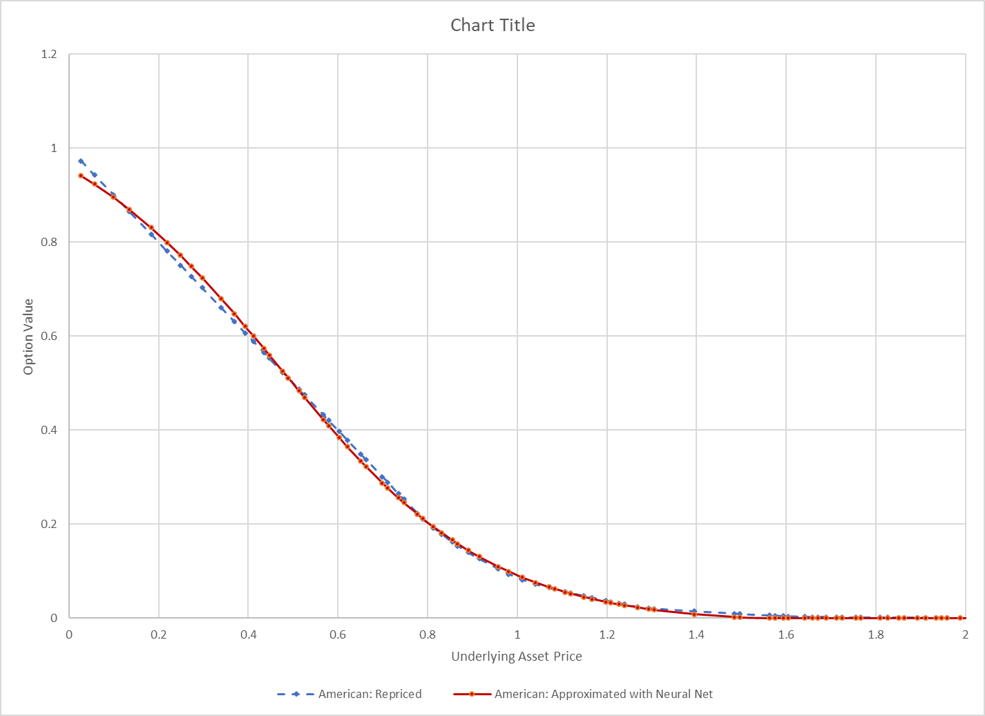
I train the model. It only takes a few seconds. I try the model on some new test data and it looks really good. The picture below compares the neural network approximation with the true value.

If your model’s done well at this point, then you can stop. If it’s not doing well, you may need to try a deeper model, or different model, or add more data. SAS offers model interpretability tools like partial dependency to help you gauge how the model fits for different variables.

Deploying the model

If you like the way this model is approximating your trade or other financial instrument values, you can deploy the model so that it can be used to run on-demand stress tests or to speed up intra-day risk estimations. There are many ways to do this in SAS. The neural network can be published to run in SAS, in data-base, in Hadoop, or in-stream with a single click. I can also access my model via REST API, which gives me lots of deployment options. What I’ll do, though, is use these models in SAS High-Performance Risk (HPRisk) so that I can leverage the risk environment for stress testing and simulation and use its nice GUI.

HPRisk lets you specify any function, or method, to value an instrument. Given the mapping of the functions to the instruments, it coordinates a massively parallel run of the portfolio valuation for stress testing or simulation.

Remember the SAS file we generated when we trained the neural network. I can throw that code into HPRisk’s method and now HPRisk will run the neural network I just trained.

I can specify a scenario through the HPRisk UI and instantly get the results of my approximation.

Considerations

I introduced this as a practical example of AI, specifically machine learning in banking, so let’s make sure we keep it practical, by considering the following:
 
    • Only approximate instruments that need it. For example, if it's a European option, don’t approximate. The function to calculate its true price, the Black-Scholes equation, already runs really fast. The whole point is that you’re trying to speed up the estimation.
 
    • Keep in mind that this is still an approximation, so only use this when you’re willing to accept some inaccuracy.
 
    • In practice, you could be training hundreds of networks depending on the types of instruments you have. You’ll want to optimize the training time of the networks by training multiple networks at once. You can do this with SAS.
 
    • The good news is that if you train the networks on a wide range of data, you probably won’t have to retrain often. They should be pretty resilient. This is a nice perk of the neural networks over the second-order approximation whereby parameters need to be recomputed often.
 
    • I’ve chosen neural networks for this example but be open to other algorithms. Note that different instruments may benefit from different algorithms. Gradient boosting and others may offer simpler, more intuitive models, that get similar accuracy.

When it comes to AI in business, you’re most likely to succeed when you have a well-defined problem, like our stress testing that takes too long or isn’t accurate. You also need good data to work with. This example had both, which made it a good candidate for to demonstrate practical AI.

More resources

Interested in other machine learning algorithms or AI technologies in general? Here are a few resources to keep learning.

Article: A guide to machine learning algorithms and their applications
Blog post: Which machine learning algorithm should I use?
Video: Supervised vs. Unsupervised Learning
Article: Five AI technologies that you need to know