At SAS, we love data. Data is central to our corporate vision: to transform a world of data into a world of intelligence. We're also famous for enjoying M&Ms, but to us they are more than a sweet snack. They're also another source of data.

My colleague Pete Privitera, with a team of like-minded "makers," built a device that they named SnackBot. SnackBot is an internet-connected sensor that measures the flow of M&Ms in a particular SAS break room. There's a lot to love about this project. You can learn more by watching its origin story in this video:

As the number of M&Ms changes, SnackBot takes a reading and records the M&M count in a database. Most readings reflect a decrease in candy pieces, as my colleagues help themselves to a treat. But once per week, the reading shows a drastic increase -- as our facilities staff restocks the canister. SnackBot has its own website. It also has its own API, and you know what that means (right?). It means that we can use SAS to read and analyze the sensor data.

Reading sensor data into SAS with the SnackBot API

The SnackBot system offers a REST API with a JSON data response. Like any REST API, we can use PROC HTTP to fetch the data, and the JSON library engine to parse the response into a SAS data set.

%let start = '20MAY2018:0:0:0'dt;
 
/* format the start/end per the API needs */
%let start_time= %sysfunc(putn(&start.,is8601dt26.));
%let end_time=   %sysfunc(datetime(),is8601dt26.);
 
/* Call the SnackBot API from snackbot.net */
filename resp temp;
proc http
  method="GET"
  url="http://snackbot.net/snackdata?start_time=&start_time.%str(&)end_time=&end_time.%str(&)utc_offset_minutes=-240"
  out=resp;
run;
 
/* JSON libname engine to read the result       */
/* Simple record layout, all in the ROOT member */
libname mms json fileref=resp;
data mmlevels;
  set mms.root;
run;

I've written about how to use SAS with REST APIs in several other blog posts, so I won't dwell on this part of the process here. This short program retrieves the raw data from SnackBot, which represents a series of M&M "levels" (count of remaining pieces) and a timestamp for each measurement. It's a good start. Though there are only two fields to work with here, there's quite a bit we can do with these data.

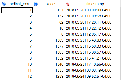
Add features to the raw sensor data

With a few additional DATA step statements and some built-in SAS formats, we can derive several interesting characteristics of these data for use in further analysis.

First, we need to convert the character-formatted datetime field to a proper SAS datetime value. That's easily achieved with the INPUT function and the ANYDTDTM informat. (Rick Wicklin wrote a helpful article about how how the ANYDT* informats work.)

data mmlevels;
  set mms.root;
  drop ordinal_root timestamp;
  /* Convert the TIMESTAMP field to native value -- it's a character */
  datetime = input(timestamp, anydtdtm.);
  date = datepart(datetime);
  time = timepart(datetime);
  dow = date;
  qhour = round(datetime,'0:15:0'T);
  format  datetime datetime20. 
          qhour datetime20.
          date date9.
          time timeampm10.
          dow downame.;
run;

For convenience, I duplicated the datetime value a few times and applied different formats so we can get different views of the same value: datetime, just the date, just the time-of-day, and the day-of-week. I also used the ROUND function to "round" the raw datetime value to the nearest quarter hour. I'll explain why I've done that in a later step, but the ROUNDing of a time value is one of the documented unusual uses of the ROUND function.

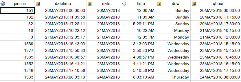
Even with this small amount of data preparation, we can begin to analyze the characteristics of these data. For example, let's look at the descriptive stats for the data classified by day-of-week:

title "SnackBot readings per day-of-week";
proc means data=mmlevels mean stddev max min;
 var pieces;
 class dow;
run;

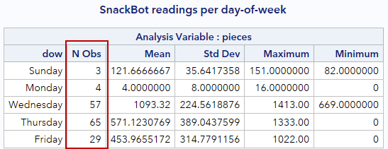
The "N Obs" column shows the number of measurements taken over the entire "study period" broken down by day-of-week. If a measurement is a proxy for a "number-of-pieces-changed" event, then we can see that most events happen on Wednesday, Thursday, and Friday. From this, can you guess which day the M&M canister is refilled?

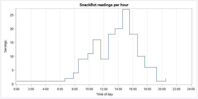
Let's take another slice through these data, but this time looking at time-of-day. For this, I used PROC FREQ to count the measurements by hour. I applied the HOUR2. format, which allows the SAS procedure to group these data into hour-long intervals with no need for additional data prep. ( I've written previously about how to use SAS formats to derive new categories without expensive data rewriting.) Then I used PROC SGPLOT to produce a step plot for the 24-hour cycle.

/* Count of readings per hour of the day */ 
title "SnackBot readings per hour";
proc freq data=mmlevels ;
 table time / out=perhour;
 format time hour2.;
run;
 
ods graphics / height=400 width=800;
 
title "SnackBot readings per hour";
proc sgplot data=perhour des="Readings per hour of day";
 step x=time y=count;
 xaxis min='0:0:0't max='24:0:0't label="Time of day" grid;
 yaxis label="Servings";
run;

From the chart, we can see that most M&M "events" happen around 11am, and then again between 2pm and 4pm. From personal experience, I can confirm that those are the times when I hear the M&Ms calling to me.

Expand the time series to regular intervals

The SnackBot website can tell you how many M&Ms are remaining right now. But what if you want to know how many were remaining last Friday? Or on any typical Monday morning?

The sensor data that we've analyzed so far is sparse -- that is, there are data entries for each "change" event, but not for every discrete time interval in the study period. I don't know how the SnackBot sensor records its readings -- it might sample the M&M levels every minute, or every second. Regardless, the API reports (and probably stores) only the records that represent a change. If SnackBot records that the final 24 pieces were depleted at 25JUN2018:07:45:00 (a Monday morning) bringing the count to 0, how many M&Ms remain at 1pm later that day? The data don't tell us explicitly with a recorded reading. But we can assume at that point that the count was still 0. The next recorded reading occurs at 27JUN2018:10:30:00 (on a Wednesday, bringing the count to 1332 -- oh joy!).

If we want to create a useful time series visualization of the M&M candy counts over time, we need to expand the time series from these sparse recordings to regular intervals. SAS offers a few sophisticated time series procedures to accomplish this: PROC EXPAND, PROC TIMESERIES, and PROC TIMEDATA. Each of these offer powerful econometrics methods for interpolation and forecasting -- and that's more than we need for this situation. For my example, I took a more low-tech approach.

First, I created an empty data set with datetime entries at quarter-hour intervals, covering the study period of the data we're looking at.

/* Empty data set with 15 minute interval slots    */
/* Regular intervals for the entire "study" period */
data timeslots;
  last = datetime();
  length qhour 8;
  format qhour datetime20;
  drop last i;
  do i = &start. to last by '0:15:00't;
    qhour = i;
    output;
  end;
run;

Then I used a DATA step to merge these empty slots with the actual event data that I had rounded to the nearest quarter hour (remember that?):

/* Merge the sample data with the timeslots */
data expand;
  merge mmlevels(keep=pieces qhour) timeslots;
  by qhour;
run;

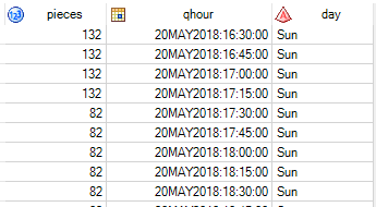
Finally, I used a variation of a last-observation-carried-forward (LOCF) approach to fill in the remaining empty slots. If a reading at 20MAY2018:11:15:00 reports 132 pieces remaining, then that value should be RETAINed for each 15-minute slot until the next reading at 20MAY2018:17:30:00. (That reading is 82 pieces -- meaning somebody helped themselves to 50 pieces. Recommended serving size for plain M&Ms is 20 pieces, but I'm not passing judgement.) I also recorded a text value for the day-of-week to help with the final visualization.

/* for empty timeslots, carry the sample data   */
/* forward, so we always have a count of pieces */
/* Variation on a LOCF technique                */
data final;
  set expand;
  length day $ 3;
  /* 3-char value for day of week */
  day=put(datepart(qhour),weekdate3.);
  retain hold;
  if not missing(pieces) then
    hold=pieces;
  else pieces=hold;
  drop hold;
  if not missing(pieces);
run;

Now I have data that represents the regular intervals that we need.

Putting it all together

For my final visualization, I created a series plot for the study period. It shows the rise and fall of M&Ms levels in one SAS break room over several weeks. For additional "color", I annotated the plot with a block chart to delineate the days of the week.

title 'Plain M&M pieces on S1 tracked by SnackBot';
ods graphics / height=300 width=1600;
 
proc sgplot data=final des='M&M pieces tracked by SnackBot';
 
  /* plot the data as a series */ 
  series x=qhour y=pieces / lineattrs=(color=navy thickness=3px);
 
  /* Yes, these are the "official" M&M colors               */
  /* Will be applied in data-order, so works best when data */
  /* begins on a Sunday                                     */
  styleattrs datacolors=(red orange yellow green blue CX593B18 red);
  /* block areas to indicate days-of-week                   */
  block x=qhour block=day / transparency=0.65
    valueattrs=(weight=bold size=10pt color=navy);
 
  xaxis minor display=(nolabel);
  yaxis display=(nolabel) grid max=1600 minor;
run;

You can see the pattern. M&Ms are typically filled on Wednesday to the canister capacity of about 1400 pieces. We usually enter into the weekend with 0 remaining, but there are exceptions. The week of May 27 was our Memorial Day holiday, which explains the lack of activity on Monday (and even Tuesday) during that week as SAS folks took advantage of a slow week with their vacation plans.

More about SAS and M&Ms data

You can download the complete code for this example from my public Gist on GitHub. The example code should work with SAS University Edition and SAS OnDemand for Academics, as well as with any SAS environment that can reach the internet with PROC HTTP.

For more M&M data fun, check out Rick Wicklin's article about the distribution of colors in plain M&Ms. SnackBot does not (yet) report on how many and which color of M&Ms are taken per serving, but using statistics, we can predict that!

Finally, I'd like to (humbly!) point out that my 2009 blog post about a snack-driven dashboard was remarkably prescient. True, I was riffing off of the idea of the internet-connected Coke machine from the 1980s, but thanks to SnackBot for making my dream come to life.