A common barrier to quantitative research, especially in health and financial areas, is the inability to share sensitive data due to confidentiality and privacy. It can be difficult and time consuming to get permission to share the data, which means useful research is delayed or not even attempted. However, collaborators seeking to develop algorithms or modeling methods may not need the real data to start working on the project, as long as an approximate, realistic data set can be used in place of the real data set. This alternative data is known as synthetic data.

Researchers could use synthetic data to, for example, understand the format of the real data, develop an understanding of its statistical properties, build preliminary models, or tune algorithm parameters. Analytical procedures and code developed using the synthetic data can then be passed to the data owner if the collaborators are not permitted to access the original data. Even if the collaborators are eventually granted access, synthetic data allow the work to be conducted in parallel with tasks required to access the real data, allowing an efficient path to the final analysis.

One method for producing synthetic data with SAS was presented at SAS Global Forum 2017 with this corresponding paper (Bogle and Erickson 2017), which implemented an algorithm originally proposed in another paper (Bogle and Mehrotra 2016, subscription required). The implementation uses the OPTMODEL procedure and solvers in SAS/OR to create synthetic data with statistical raw moments similar to the real data.

Moments

Most SAS users are familiar with mean, variance, and covariance. The mean is the first-order raw moment, $\mathbf{E}[X]$. The variance is the second-order marginal central moment, $\mathbf{E}[(X-\mathbf{E}[X])^2]$, and covariance is the second-order mixed central moment, $\mathbf{E}[(X-\mathbf{E}[X])(Y-\mathbf{E}[Y])]$. Skewness and kurtosis are the third- and fourth-order normalized moments.

This method considers only raw moments, which keeps the optimization problem linear. The more of these moments that are matched, the more like the original data it will be. It is difficult to match the moments exactly, so the algorithm tries to keep them within desired bounds. For example, one of the fourth-order moments (meaning the sum of the exponents is four) could be $\mathbf{E}[X^2YZ]$, which could have a value of 0.5 in the real data set. The method might try to "match" this moment by constraining that moment in the new data set to be between 0.48 and 0.52. If $N$ observations are desired, this would ideally mean that the moment value would be constrained between those bounds, $\displaystyle{0.48 \le \frac{1}{N} \sum_{i=1}^N x_i^2y_iz_i \le 0.52}$.

There are a couple of problems with solving a system of inequalities like this. First, it is not linear or convex, so it would be very hard to solve, especially when some variables need to take integer values. This macro instead creates candidate observations and uses mathematical optimization to select which observations to include. Second, there might not be a solution that solves such a system of inequalities, so the method allows violations to the bounds on the moments and minimizes them.

Algorithm

There are three basic steps to the algorithm. The first step reads in the original data, computes the upper and lower bounds on the moments, and sets up other parameters for the optimization models. The second step uses column generation with a linear program to produce candidate synthetic observations. The third step uses an integer program to select the desired number of synthetic observations from the candidate synthetic observations, while minimizing the largest scaled violation of the moment bounds. The following code is the macro that generates synthetic data by calling a different macro for each of the three steps.

%macro GENDATA(INPUTDATA, METADATA, OUTPUTDATA=SyntheticData,
   MOMENTORDER=3, NUMOBS=0, MINNUMIPCANDS=0, LPBATCHSIZE=10, LPGAP=1E-3,
   NUMCOFORTHREADS=1, MILPMAXTIME=600, RELOBJGAP=1E-4, ALPHA=0.95,
   RANDSEED=0);
   proc optmodel printlevel=0;
      call streaminit(&RANDSEED);
      %PRELIMINARYSTEP(INPUTDATA=&INPUTDATA, METADATA=&METADATA,
         MOMENTORDER=&MOMENTORDER, ALPHA=&ALPHA);
      %LPSTEP(MOMENTORDER=&MOMENTORDER, NUMOBS=&NUMOBS,
         MINNUMIPCANDS=&MINNUMIPCANDS, LPBATCHSIZE=&LPBATCHSIZE,
         LPGAP=&LPGAP, NUMCOFORTHREADS=&NUMCOFORTHREADS);
      %IPSTEP(OUTPUTDATA=&OUTPUTDATA, MOMENTORDER=&MOMENTORDER,
         NUMOBS=&NUMOBS, MINNUMIPCANDS=&MINNUMIPCANDS,
         MILPMAXTIME=&MILPMAXTIME, RELOBJGAP=&RELOBJGAP);
   quit;
%mend GENDATA;

You can see that there are several parameters, which are described in the paper. Most of them control the balance of the quality of the synthetic data with the time needed to produce the synthetic data.

PROC OPTMODEL Features

The macro demonstrates some useful features of PROC OPTMODEL. One option for the macro is to use PROC OPTMODEL's COFOR loop. This allows multiple LPs to be solved concurrently, which can speed up the LP step. The implementation breaks the assignment of creating candidate observations into NUMCOFORTHREADS groups, and one solve statement from each group can be run concurrently. The use of COFOR reduces the total time from five hours to three hours in the example below.

The code also calls SAS functions not specific to PROC OPTMODEL, including RAND, STD, and PROBIT. The RAND function is used to create random potential observations during the column generation process. The STD and PROBIT functions are used to determine the desired moment range based on the input data and a user-specified parameter.

Example

The examples in the paper are based on the Sashelp.Heart data set. The data set is modified to fit the requirements that all variables must be numeric and there can be no missing data.

The example randomly divides the data into Test and Training data sets so that a model based on the Training data set can be tested against a model based on a synthetic data set derived from the Training data set.

The following call of the macro generates the synthetic data based on the Training data set with the appropriate METADATA data set. It allows up to four LPs to be solved concurrently, matches moments up to the third order, allows 20 minutes for the MILP solver, and uses a fairly small range for the moment bounds.

%GENDATA(INPUTDATA=Training, METADATA=Metadata, NUMCOFORTHREADS=4,
   MOMENTORDER=3, MILPMAXTIME=1200, ALPHA=0.2);

One way to verify that the synthetic data are similar to the real data is to compare the means, standard deviations, and covariances of the input and synthetic data sets. The paper shows how to do this using PROC MEANS and PROC CORR on a smaller synthetic data set.

In this case we want to compare the training and synthetic data by comparing how well the models they fit score the Test data set. One of the variables indicates if a person is dead, so we can use a logistic regression to predict if a person is dead or alive. Because BMI is a better health predictor than height or weight, we have added a BMI column to the data sets. The following code calls PROC LOGISTIC for the two data sets.

proc logistic data=TrainingWithBmi; 
   model Dead = Male AgeAtStart Diastolic Systolic Smoking Cholesterol BMI / outroc=troc; 
   score data=TestingWithBmi out=valpred outroc=vroc; 
run; 
proc logistic data=SyntheticDataWithBmi; 
   model Dead = Male AgeAtStart Diastolic Systolic Smoking Cholesterol BMI / outroc=troc; 
   score data=TestingWithBmi out=valpred outroc=vroc; 
run;

This produces quite a bit of output. One useful comparison is the area under the curve (AUC) of the ROC curve, which plots a comparison of sensitivity and specificity of the model. The first plot is for the original training data scored with the testing data from the original data set. The second plot is for the synthetic data scored with the testing data from the original data set. You can see that the curves are fairly similar and there is little difference between the AUCs.

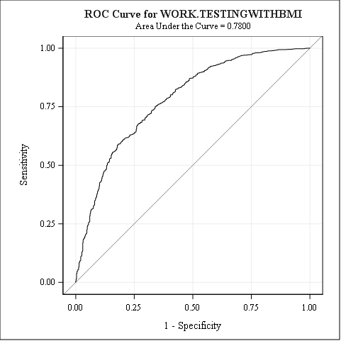
This synthetic data set behaves similarly to the original data set and can be safely shared without risk of exposing personally identifiable information.

What uses do you have for synthetic data?