This is the third and last introductory article about how to bootstrap time series in SAS. In the first article, I presented the simple block bootstrap and discussed why bootstrapping a time series is more complicated than for regression models that assume independent errors. Briefly, when you perform residual resampling
Tag: Statistical Programming
As I discussed in a previous article, the simple block bootstrap is a way to perform a bootstrap analysis on a time series. The first step is to decompose the series into additive components: Y = Predicted + Residuals. You then choose a block length (L) that divides the total
On The DO Loop blog, I write about a diverse set of topics, including statistical data analysis, machine learning, statistical programming, data visualization, simulation, numerical analysis, and matrix computations. In a previous article, I presented some of my most popular blog posts from 2020. The most popular articles often deal
When you perform a linear regression, you can examine the R-square value, which is a goodness-of-fit statistic that indicates how well the response variable can be represented as a linear combination of the explanatory variables. But did you know that you can also go the other direction? Given a set
Do you know that you can create a vector that has a specific correlation with another vector? That is, given a vector, x, and a correlation coefficient, ρ, you can find a vector, y, such that corr(x, y) = ρ. The vectors x and y can have an arbitrary number
To help visualize regression models, SAS provides the EFFECTPLOT statement in several regression procedures and in PROC PLM, which is a general-purpose procedure for post-fitting analysis of linear models. When scoring and visualizing a model, it is important to use reasonable combinations of the explanatory variables for the visualization. When
Intuitively, the skewness of a unimodal distribution indicates whether a distribution is symmetric or not. If the right tail has more mass than the left tail, the distribution is "right skewed." If the left tail has more mass, the distribution is "left skewed." Thus, estimating skewness requires some estimates about
The expected value of a random variable is essentially a weighted mean over all possible values. You can compute it by summing (or integrating) a probability-weighted quantity over all possible values of the random variable. The expected value is a measure of the "center" of a probability distribution. You can
A fundamental principle of data analysis is that a statistic is an estimate of a parameter for the population. A statistic is calculated from a random sample. This leads to uncertainty in the estimate: a different random sample would have produced a different statistic. To quantify the uncertainty, SAS procedures
A previous article shows how to use a recursive formula to compute exact probabilities for the Poisson-binomial distribution. The recursive formula is an O(N2) computation, where N is the number of parameters for the Poisson-binomial (PB) distribution. If you have a distribution that has hundreds (or even thousands) of parameters,