When you perform a linear regression, you can examine the R-square value, which is a goodness-of-fit statistic that indicates how well the response variable can be represented as a linear combination of the explanatory variables. But did you know that you can also go the other direction? Given a set of explanatory variables and an R-square statistic, you can create a response variable, Y, such that a linear regression of Y on the explanatory variables produces exactly that R-square value.

The geometry of correlation and least-square regression

In a previous article, I showed how to compute a vector that has a specified correlation with another vector. You can generalize that situation to obtain a vector that has a specified relationship with a linear subspace that is spanned by multiple vectors.

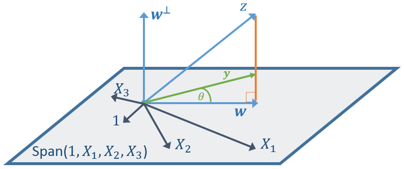
Recall that the correlation is related to the angle between two vectors by the formula cos(θ) = ρ, where θ is the angle between the vectors and ρ is the correlation coefficient. Therefore, correlation and "angle between" measure similar quantities. It makes sense to define the angle between a vector and a linear subspace as the smallest angle the vector makes with any vector in the subspace. Equivalently, it is the angle between the vector and its (orthogonal) projection onto the subspace.

This is shown graphically in the following figure. The vector z is not in the span of the explanatory variables. The vector w is the projection of z onto the linear subspace. As explained in the previous article, you can find a vector y such that the angle between y and w is θ, where cos(θ) = ρ. Equivalently, the correlation between y and w is ρ.

Correlation between a response vector and a predicted vector

There is a connection between this geometry and the geometry of least-squares regression. In least-square regression, the predicted response is the projection of an observed response vector onto the span of the explanatory variables. Consequently, the previous article shows how to simulate an "observed" response vector that has a specified correlation with the predicted response.

For simple linear regression (one explanatory variable), textbooks often point out that the R-square statistic is the square of the correlation between the independent variable, X, and the response variable, Y. So, the previous article enables you to create a response variable that has a specified R-square value with one explanatory variable.

The generalization to multivariate linear regression is that the R-square statistic is the square of the correlation between the predicted response and the observed response. Therefore, you can use the technique in this article to create a response variable that has a specified R-square value in a linear regression model.

To be explicit, suppose you are given explanatory variables X₁, X₂, ..., X_k, and a correlation coefficient, ρ. The following steps generate a response variable, Y, such that the R-square statistic for the regression of Y onto the explanatory variables is ρ²:

1. Start with an arbitrary guess, z.
2. Use least-squares regression to find w = $\hat{\mathbf{z}}$, which is the projection of z onto the subspace spanned by the explanatory variables and the 1 vector.
3. Use the technique in the previous article to find Y such that corr(Y, w) = ρ

Create a response variable that has a specified R-square value in SAS

The following program shows how to carry out this algorithm in the SAS/IML language:

proc iml;
/* Define or load the modules from 
   https://blogs.sas.com/content/iml/2020/12/17/generate-correlated-vector.html
*/
load module=_all_;
/* read some data X1, X2, ... into columns of a matrix, X */
use sashelp.class;
   read all var {"Height" "Weight" "Age"} into X;  /* read data into (X1,X2,X3) */
close;
 
/* Least-squares fit = Project Y onto span(1,X1,X2,...,Xk) */
start OLSPred(y, _x);
   X = j(nrow(_x), 1, 1) || _x;
   b = solve(X`*X, X`*y);
   yhat = X*b;
   return yhat;
finish;
 
/* specify the desired correlation between Y and \hat{Y}. Equiv: R-square = rho^2 */
rho = 0.543;        
 
call randseed(123);
guess = randfun(nrow(X), "Normal");   /* 1. make random guess */
w = OLSPred(guess, X);                /* 2. w is in Span(1,X1,X2,...) */
Y = CorrVec1(w, rho, guess);          /* 3. Find Y such that corr(Y,w) = rho   */
/* optional: you can scale Y anyway you want ... */
/* in regression, R-square is squared correlation between Y and YHat */
corr = corr(Y||w)[2];
R2 = rho**2;                          
PRINT rho corr R2;

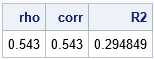
The program uses a random guess to generate a vector Y such that the correlation between Y and the least-squares prediction for Y is exactly 0.543. In other words, if you run a regression model where Y is the response and (X1, X2, X3) are the explanatory variables, the R-square statistic for the model will be ρ² = 0.2948. Let's write the Y variable to a SAS data set and run PROC REG to verify this fact:

/* Write to a data set, then call PROC REG */
Z = Y || X;
create SimCorr from Z[c={Y X1 X2 X3}];
append from Z;
close;
QUIT;
 
proc reg data=SimCorr plots=none;
   model Y = X1 X2 X3;
   ods select FitStatistics ParameterEstimates;
quit;

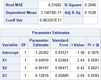
The "FitStatistics" table that is created by using PROC REG verifies that the R-square statistic is 0.2948, which is the square of the ρ value that was specified in the SAS/IML program. The ParameterEstimates table from PROC REG shows the vector in the subspace that has correlation ρ with Y. It is -1.26382 + 0.04910*X1 - 0.00197*X2 - 0.12016 *X3.

Summary

Many textbooks point out that the R-square statistic in multivariable regression has a geometric interpretation: It is the squared correlation between the response vector and the projection of that vector onto the linear subspace of the explanatory variables (which is the predicted response vector). You can use the program in this article to solve the inverse problem: Given a set of explanatory variables and correlation, you can find a response variable for which the R-square statistic is exactly the squared correlation.

You can download the SAS program that computes the results in this article.