A fundamental principle of data analysis is that a statistic is an estimate of a parameter for the population. A statistic is calculated from a random sample. This leads to uncertainty in the estimate: a different random sample would have produced a different statistic. To quantify the uncertainty, SAS procedures often support options that estimate standard errors for statistics and confidence intervals for parameters.

Of course, if statistics have uncertainty, so, too, do functions of the statistics. For complicated functions of the statistics, the bootstrap method might be the only viable technique for quantifying the uncertainty.

This article shows how to obtain confidence intervals for the eigenvalues of a correlation matrix. The eigenvalues are complicated functions of the correlation estimates. The eigenvalues are used in a principal component analysis (PCA) to decide how many components to keep in a dimensionality reduction. There are two main methods to estimate confidence intervals for eigenvalues: an asymptotic (large sample) method, which assumes that the eigenvalues are multivariate normal, and a bootstrap method, which makes minimal distributional assumptions.

The following sections show how to compute each method. A graph of the results is shown to the right. For the data in this article, the bootstrap method generates confidence intervals that are more accurate than the asymptotic method.

This article was inspired by Larsen and Warne (2010), "Estimating confidence intervals for eigenvalues in exploratory factor analysis." Larsen and Warne discuss why confidence intervals can be useful when deciding how many principal components to keep.

Eigenvalues in principal component analysis

To demonstrate the techniques, let's perform a principal component analysis (PCA) on the four continuous variables in the Fisher Iris data. In SAS, you can use PROC PRINCOMP to perform a PCA, as follows:

%let DSName = Sashelp.Iris;
%let VarList = SepalLength SepalWidth PetalLength PetalWidth;
 
/* 1. compute value of the statistic on original data */
proc princomp data=&DSName STD plots=none;     /* stdize PC scores to unit variance */
   var &VarList;
   ods select ScreePlot Eigenvalues NObsNVar;
   ods output Eigenvalues=EV0 NObsNVar=NObs(where=(Description="Observations"));
run;
 
proc sql noprint;                              
 select nValue1 into :N from NObs;   /* put the number of obs into macro variable, N */
quit;
%put &=N;

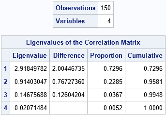
The first table shows that there are 150 observations. The second table displays the eigenvalues for the sample, which are 2.9, 0.9, 0.15, and 0.02. If you want a graph of the eigenvalues, you can use the PLOTS(ONLY)=SCREE option on the PROC PRINCOMP statement. The ODS output statement creates SAS data set from the tables. The PROC SQL call creates a macro variable, N, that contains the number of observations.

Asymptotic confidence intervals

If a sample size, n, is large enough, the sampling distribution of the eigenvalues is approximately multivariate normal (Larsen and Ware (2010, p. 873)). If g is an eigenvalue for a correlation matrix, then an asymptotic confidence interval is
     g ± z^* sqrt( 2 g² / n )
where z^* is the standard normal quantile, as computed in the following program:

/* Asymptotic CIs for eigenvalues (Larsen and Warne (2010, p. 873) */
data AsympCI;
set EV0;
alpha = 0.05;
z = quantile("Normal", 1 - alpha/2);  /* = 1.96 */
SE = sqrt(2*Eigenvalue**2 / &N);
Normal_LCL = Eigenvalue - SE;         /* g +/- z* sqrt(2 g^2 / n) */
Normal_UCL = Eigenvalue + SE;
drop alpha z SE;
run;
 
proc print data=AsympCI noobs;
   var Number Eigenvalue Normal_LCL Normal_UCL;
run;

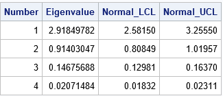
The lower and upper confidence limits are shown for each eigenvalue. The advantage of this method is its simplicity. The intervals assume that the distribution of the eigenvalues is multivariate normal, which will occur when the sample size is very large. Since N=150 does not seem "very large," it is not clear whether these confidence intervals are valid. Therefore, let's estimate the confidence intervals by using the bootstrap method and compare the bootstrap intervals to the asymptotic intervals.

Bootstrap confidence intervals for eigenvalues

The bootstrap computations in this section follow the strategy outlined in the article "Compute a bootstrap confidence interval in SAS." (For additional bootstrap tips, see "The essential guide to bootstrapping in SAS.") The main steps are:

1. Compute a statistic for the original data. This was done in the previous section.
2. Use PROC SURVEYSELECT to resample (with replacement) B times from the data. For efficiency, put all B random bootstrap samples into a single data set.
3. Use BY-group processing to compute the statistic of interest on each bootstrap sample. The union of the statistics is the bootstrap distribution, which approximates the sampling distribution of the statistic. Remember to turn off ODS when you run BY-group processing!
4. Use the bootstrap distribution to obtain confidence intervals for the parameters.

The steps are implemented in the following SAS program:

/* 2. Generate many bootstrap samples */
%let NumSamples = 5000;       /* number of bootstrap resamples */
proc surveyselect data=&DSName NOPRINT seed=12345
     out=BootSamp(rename=(Replicate=SampleID))
     method=urs              /* resample with replacement */
     samprate=1              /* each bootstrap sample has N observations */
     /* OUTHITS                 option to suppress the frequency var */
     reps=&NumSamples;       /* generate NumSamples bootstrap resamples */
run;
 
/* 3. Compute the statistic for each bootstrap sample */
/* Suppress output during this step:
   https://blogs.sas.com/content/iml/2013/05/24/turn-off-ods-for-simulations.html
*/
%macro ODSOff();   ods graphics off; ods exclude all;  ods noresults;   %mend;
%macro ODSOn();    ods graphics on;  ods exclude none; ods results;     %mend;
 
%ODSOff;
proc princomp data=BootSamp STD plots=none;
   by SampleID;
   freq NumberHits;
   var &VarList;
   ods output Eigenvalues=EV(keep=SampleID Number Eigenvalue);
run;
%ODSOn;
 
/* 4. Estimate 95% confidence interval as the 2.5th through 97.5th percentiles of boostrap distribution */
proc univariate data=EV noprint;
   class Number;
   var EigenValue;
   output out=BootCI pctlpre=Boot_ pctlpts=2.5  97.5  pctlname=LCL UCL;
run;
 
/* merge the bootstrap CIs with the normal CIs for comparison */
data AllCI;
   merge AsympCI(keep=Number Eigenvalue Normal:) BootCI(keep=Number Boot:);
   by Number;
run;
 
proc print data=AllCI noobs;
   format Eigenvalue Normal: Boot: 5.3;
run;

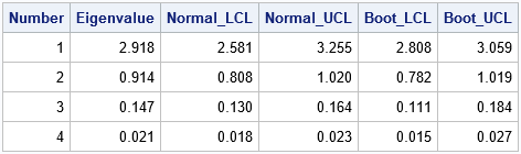
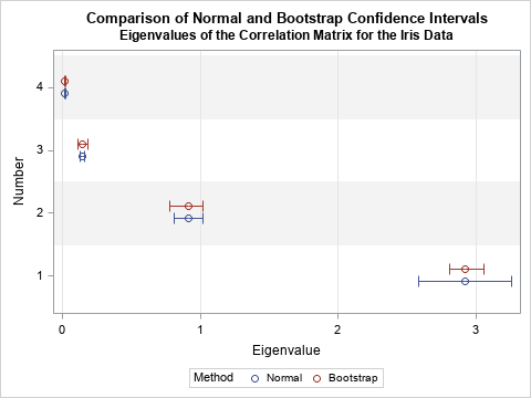
The table displays the bootstrap confidence intervals (columns 5 and 6) next to the asymptotic confidence intervals (columns 3 and 4). It is easier to compare the intervals if you visualize them graphically, as follows:

/* convert from wide to long */
data CIPlot;
   set AllCI;
   Method = "Normal   "; LCL = Normal_LCL; UCL = Normal_UCL; output;
   Method = "Bootstrap"; LCL = Boot_LCL; UCL = Boot_UCL; output;
   keep Method Eigenvalue Number LCL UCL;
run;
 
title "Comparison of Normal and Bootstrap Confidence Intervals";
title2 "Eigenvalues of the Correlation Matrix for the Iris Data";
ods graphics / width=480px height=360px;
proc sgplot data=CIPlot;
   scatter x=Eigenvalue y=Number / group=Method clusterwidth=0.4
           xerrorlower=LCL xerrorupper=UCL groupdisplay=cluster;
   yaxis grid type=discrete colorbands=even colorbandsattrs=(color=gray transparency=0.9);
   xaxis grid;
run;

The graph is shown at the top of this article. The graph nicely summarizes the comparison. For the first (largest) eigenvalue, the bootstrap confidence interval is about half as wide as the normal confidence interval. Thus, the asymptotic result seems too wide for these data. For the other eigenvalues, the normal confidence intervals appear to be too narrow.

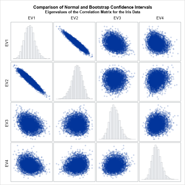
If you graph the bootstrap distribution, you can see that the bootstrap distribution does not appear to be multivariate normal. This presumably explains why the asymptotic intervals are so different from the bootstrap intervals. For completeness, the following graph shows a matrix of scatter plots and marginal histograms for the bootstrap distribution. The histograms indicate skewness in the bootstrap distribution.

Summary

This article shows how to compute confidence intervals for the eigenvalues of an estimated correlation matrix. The first method uses a formula that is valid when the sampling distribution of the eigenvalues is multivariate normal. The second method uses bootstrapping to approximate the distribution of the eigenvalues, then uses percentiles of the distribution to estimate the confidence intervals. For the Iris data, the bootstrap confidence intervals are substantially different from the asymptotic formula.