Last week I blogged about the broken-stick problem in probability, which reminded me that the broken-stick model is one of the many techniques that have been proposed for choosing the number of principal components to retain during a principal component analysis. Recall that for a principal component analysis (PCA) of p variables, a goal is to represent most of the variation in the data by using k new variables, where hopefully k is much smaller than p. Thus PCA is known as a dimension-reduction algorithm.

Many researchers have proposed methods for choosing the number of principal components. Some methods are heuristic, others are statistical. No method is perfect. Often different techniques result in different suggestions.

This article uses SAS to implement the broken stick model and compares that method with three other simple rules for dimension reduction. A few references are provided at the end of this article.

A principal component analysis by using PROC PRINCOMP

Let's start with an example. In SAS, you can use the PRINCOMP procedure to conduct a principal component analysis. The following example is taken from the Getting Started example in the PROC PRINCOMP documentation. The program analyzes seven crime rates for the 50 US states in 1977. (The documentation shows how to generate the data set.) The following call generates a scree plot, which shows the proportion of variance explained by each component. It also writes the Eigenvalues table to a SAS data set:

proc princomp data=Crime plots=scree;
   var Murder Rape Robbery Assault Burglary Larceny Auto_Theft;
   id State;
   ods output Eigenvalues=Evals;
run;

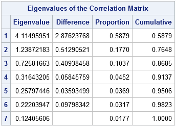
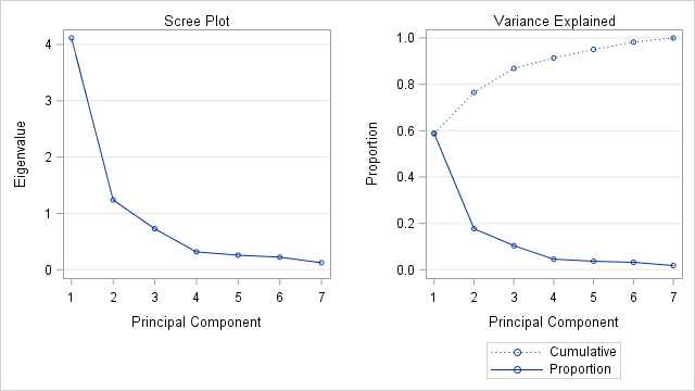
The panel shows two graphs that plot the numbers in the "Eigenvalues of the Correlation Matrix" table. The plot on the left is the scree plot, which is a graph of the eigenvalues. The sum of the eigenvalues is 7, which is the number of variables in the analysis. If you divide each eigenvalue by 7, you obtain the proportion of variance that each principal component explains. The graph on the right plots the proportions and the cumulative proportions.

The scree plot as a guide to retaining components

The scree plot is my favorite graphical method for deciding how many principal components to keep. If the scree plot contains an "elbow" (a sharp change in the slopes of adjacent line segments), that location might indicate a good number of principal components (PCs) to retain. For this example, the scree plot shows a large change in slopes at the second eigenvalue and a smaller change at the fourth eigenvalue. From the graph of the cumulative proportions, you can see that the first two PCs explain 76% of the variance in the data, whereas the first four PCs explain 91%.

If "detect the elbow" is too imprecise for you, a more precise algorithm is to start at the right-hand side of the scree plot and look at the points that lie (approximately) on a straight line. The leftmost point along the trend line indicates the number of components to retain. (In geology, "scree" is rubble at the base of a cliff; the markers along the linear trend represent the rubble that can be discarded.) For the example data, the markers for components 4–7 are linear, so components 1–4 would be kept. This rule (and the scree plot) was proposed by Cattell (1966) and revised by Cattell and Jaspers (1967).

How does the broken-stick model choose components?

D. A. Jackson (1993) says that the broken-stick method is one of the better methods for choosing the number of PCs. The method provides "a good combination of simplicity of calculation and accurate evaluation of dimensionality relative to the other statistical approaches" (p. 2212). The broken-stick model retains components that explain more variance than would be expected by randomly dividing the variance into p parts. As I discussed last week, if you randomly divide a quantity into p parts, the expected proportion of the kth largest piece is (1/p)Σ(1/i) where the summation is over the values i=k..p. For example, if p=7 then
E1 = (1 + 1/2 + 1/3 + 1/4 + 1/5 + 1/6 + 1/7) / 7 = 0.37,
E2 = (1/2 + 1/3 + 1/4 + 1/5 + 1/6 + 1/7) / 7 = 0.228,
E3 = (1/3 + 1/4 + 1/5 + 1/6 + 1/7) / 7 = 0.156, and so forth.

I think of the "expected proportions" as corresponding to a null model that contains uncorrelated (noise) variables. If you plot the eigenvalues of the correlation matrix against the broken-stick proportions, the observed proportions that are higher than the expected proportions indicate which principal components to keep.

The broken-stick model for retaining components

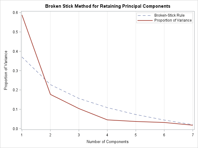
The plot to the right shows the scree plot overlaid on a dashed curve that indicates the expected proportions that result from a broken-stick model. An application of the broken-stick model keeps one PC because only the first observed proportion of variance is higher than the corresponding broken-stick proportion.

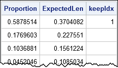
How can you compute the points on the dashed curve? The expected proportions in the broken-stick model for p variables are proportional to the cumulative sums of the sequence of ratios {1/p, 1/(p-1), ..., 1}. You can use the CUSUM function in SAS/IML to compute a cumulative sum of a sequence, as shown below. Notice that the previous call to PROC PRINCOMP used the ODS OUTPUT statement to create a SAS data set that contains the values in the Eigenvalue table. The SAS/IML program reads in that data and compares the expected proportions to the observed proportions. The number of components to retain is computed as the largest integer k for which the first k components each explain more variance than the broken-stick model (null model).

proc iml;
use Evals;  read all var {"Number" "Proportion"};  close;
 
/* Broken Stick (Joliffe 1986; J. E. Jackson, p. 47) */
/* For random p-1 points in [0,1], expected lengths of the p subintervals are: */
p = nrow(Proportion);
g = cusum(1 / T(p:1)) / p;   /* expected lengths of intervals (smallest to largest) */
ExpectedLen = g[p:1];        /* reverse order: largest to smallest */
 
keep = 0;                    /* find first k for which ExpectedLen[i] < Proportion[i] if i<=k */
do i = 1 to p while(ExpectedLen[i] < Proportion[i]);
   keep = i;
end;
print Proportion ExpectedLen keep;

As seen in the graph, only the first component is retained under the broken-stick model.

Average of eigenvalues

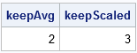
The average-eigenvalue test (Kaiser-Guttman test) retains the eigenvalues that exceed the average eigenvalue. For a p x p correlation matrix, the sum of the eigenvalues is p, so the average value of the eigenvalues is 1. To account for sampling variability, Jolliffe (1972) suggested a more liberal criterion: retain eigenvalues greater than 0.7 times the average eigenvalue. These two suggestions are implemented below:

/* Average Root (Kaiser 1960; Guttman 1954; J. E. Jackson, p. 47) */
mean = mean(Proportion);
keepAvg = loc( Proportion >= mean )[<>];
 
/* Scaled Average Root (Joliffe 1972; J. E. Jackson, p. 47-48) */
keepScaled = loc( Proportion >= 0.7*mean )[<>];
print keepAvg keepScaled;

Create the broken-stick graph

For completeness, the following statement write the broken-stick proportions to a SAS data set and call PROC SGPLOT to overlay the proportion of variance for the observed data on the broken-stick model:

/* write expected proportions for broken-stick model */
create S var {"Number" "Proportion" "ExpectedLen"}; append; close;
quit;
 
title "Broken Stick Method for Retaining Principal Components";
proc sgplot data=S;
label ExpectedLen = "Broken-Stick Rule"  Proportion = "Proportion of Variance"
      Number = "Number of Components";
   series x=Number y=ExpectedLen / lineattrs=(pattern=dash);
   series x=Number y=Proportion / lineattrs=(thickness=2);
   keylegend / location=inside position=topright across=1;
   xaxis grid;
   yaxis label = "Proportion of Variance";
run;

Summary

Sometimes people ask why PROC PRINCOMP doesn't automatically choose the "correct" number of PCs to use for dimension reduction. This article describes four popular heuristic rules, all which give different answers! The rules in this article are the scree test (2 or 4 components), the broken-stick rule (1 component), the average eigenvalue rule (2 components), and the scaled eigenvalue rule (3 components).

So how should a practicing statistician decide how many PCs to retain? First, remember that these guidelines do not tell you how many components to keep, they merely make suggestions. Second, recognize that any reduction of dimension requires a trade-off between accuracy (high dimensions) and interpretability (low dimensions). Third, these rules—although helpful—cannot replace domain-specific knowledge of the data. Try each suggestion and see if the resulting model contains the features in the data that are important for your analysis.

Further reading

• Jackson, J. E. (1991), A User’s Guide to Principal Components, New York: John Wiley & Sons.
• Jackson, D. A. (1993), "Stopping Rules in Principal Components Analysis: A Comparison of Heuristical and Statistical Approaches," Ecology, 74(8).
• Cangelosi, R. and Goriely, A. (2007), "Component retention in principal component analysis with application to cDNA microarray data," Biology Direct, 2(2).