Horn's method: A simulation-based method for retaining principal components

One purpose of principal component analysis (PCA) is to reduce the number of important variables in a data analysis. Thus, PCA is known as a dimension-reduction algorithm. I have written about four simple rules for deciding how many principal components (PCs) to keep.

There are other methods for deciding how many PCs to keep. Recently a SAS customer asked about a method known as Horn's method (Horn, 1965), also called parallel analysis. This is a simulation-based method for deciding how many PCs to keep. If the original data consists of N observations and p variables, Horn's method is as follows:

Generate B sets of random data with N observations and p variables. The variables should be normally distributed and uncorrelated. That is, the data matrix, X, is a random sample from a multivariate normal (MVN) distribution with an identity correlation parameter: X ~ MVN(0, I(p)).
Compute the corresponding B correlation matrices and the eigenvalues for each correlation matrix.
Estimate the 95th percentile of each eigenvalue distribution. That is, estimate the 95th percentile of the largest eigenvalue, the 95th percentile of the second largest eigenvalue, and so forth.
Compare the observed eigenvalues to the 95th percentiles of the simulated eigenvalues. If the observed eigenvalue is larger, keep it. Otherwise, discard it.

I do not know why the adjective "parallel" is used for Horn's analysis. Nothing in the analysis is geometrically parallel to anything else. Although you can use parallel computations to perform a simulation study, I doubt Horn was thinking about that in 1965. My best guess is that is Horn's method is a secondary analysis that is performed "off to the side" or "in parallel" to the primary principal component analysis.

Parallel analysis in SAS

You do not need to write your own simulation method to use Horn's method (parallel analysis). Horn's parallel analysis is implemented in SAS (as of SAS/STAT 14.3 in SAS 9.4M5) by using the PARALLEL option in PROC FACTOR. The following call to PROC FACTOR uses data about US crime rates. The data are from the Getting Started example in PROC PRINCOMP.

proc factor data=Crime method=Principal 
   parallel(nsims=1000 seed=54321) nfactors=parallel plots=parallel;
   var Murder Rape Robbery Assault Burglary Larceny Auto_Theft;
run;

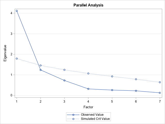
The PLOTS=PARALLEL option creates the visualization of the parallel analysis. The solid line shows the eigenvalues for the observed correlation matrix. The dotted line shows the 95th percentile of the simulated data. When the observed eigenvalue is greater than the corresponding 95th percentile, you keep the factor. Otherwise, you discard the factor. The graph shows that only one principal component would be kept according to Horn's method. This graph is a variation of the scree plot, which is a plot of the observed eigenvalues.

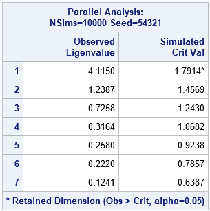
The same information is presented in tabular form in the "ParallelAnalysis" table. The first row is the only row for which the observed eigenvalue is greater than the 95th percentile (the "critical value") of the simulated eigenvalues.

Interpretation of the parallel analysis

Statisticians often use statistical tests based on a null hypothesis. In Horn's method, the simulation provides the "null distribution" of the eigenvalues of the correlation matrix under the hypothesis that the variables are uncorrelated. Horn's method says that we should only accept a factor as important if it explains more variance than would be expected from uncorrelated data.

Although the PARALLEL option is supported in PROC FACTOR, some researchers suggest that parallel analysis is valid only for PCA. Saccenti and Timmerman (2017) write, "Because Horn’s parallel analysis is associated with PCA, rather than [common factor analysis], its use to indicate the number of common factors is inconsistent (Ford, MacCallum, & Tait, 1986; Humphreys, 1975)." I an expert in factor analysis, but a basic principle of simulation is to ensure that the "null distribution" is appropriate to the analysis. For PCA, the null distribution in Horn's method (eigenvalues of a sample correlation matrix) is appropriate. However, in some common factor models, the important matrix is a "reduced correlation matrix," which does not have 1s on the diagonal.

The advantages of knowing how to write a simulation

Although the PARALLEL option in PROC FACTOR runs a simulation and summarizes the results, there are several advantages to implementing a parallel analysis yourself. For example, you can perform the analysis on the covariance (rather than correlation) matrix. Or you can substitute a robust correlation matrix as part of a robust principal component analysis.

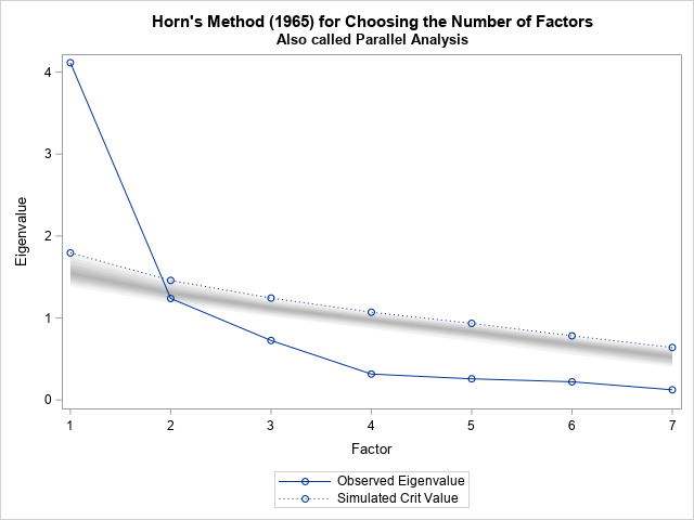
I decided to run my own simulation because I was curious about the distribution of the eigenvalues. The graph that PROC FACTOR creates shows only the upper 95th percentiles of the eigenvalue distribution. I wanted to overlay a confidence band that indicates the distribution of the eigenvalues. The band would visualize the uncertainty in the eigenvalues of the simulated data. How wide is the band? Would you get different results if you use the median eigenvalue instead of the 95th percentile?

Such a graph is shown to the right. The confidence band was created by using a technique similar to the one I used to visualize uncertainty in predictions for linear regression models. The graph shows that the distribution of each eigenvalue and connects them with a straight line. The confidence band fits well with the existing graph, even though the X axis is discrete.

Implement Horn's simulation method

Here's an interesting fact about the simulation in Horn's method. Most implementations generate B random samples, X ~ MVN(0, I(p)), but you don't actually NEED the random samples! All you need are the correlation matrices for the random samples. It turns out that you can simulate the correlation matrices directly by using the Wishart distribution. SAS/IML software includes the RANDWISHART function, which simulates matrices from the Wishart distribution. You can transform those matrices into correlation matrices, find the eigenvalues, and compute the quantiles in just a few lines of PROC IML:

/* Parallel Analysis (Horn 1965) */
proc iml;
/* 1. Read the data and compute the observed eigenvalues of the correlation */
varNames = {"Murder" "Rape" "Robbery" "Assault" "Burglary" "Larceny" "Auto_Theft"};
use Crime;
   read all var varNames into X;
   read all var "State";
close;
p = ncol(X);
N = nrow(X);
 
m = corr(X);                  /* observed correlation matrix */
Eigenvalue = eigval(m);       /* observed eigenvalues */
 
/* 2. Generate random correlation matrices from MVN(0,I(p)) data
      and compute the eigenvalues. Each row of W is a p x p scatter 
      matrix for a random sample of size N where X ~ MVN(0, I(p)) */
nSim = 1000;
call randseed(12345);
W = RandWishart(nSim, N-1, I(p));  /* each row stores a p x p matrix */
S = W / (N-1);                /* rescale to form covariance matrix */
simEigen = j(nSim, p);        /* store eigenvalues in rows */
do i = 1 to nSim;
   cov = shape(S[i,], p, p);  /* reshape the i_th row into p x p */
   R = cov2corr(cov);         /* i_th correlation matrix */
   simEigen[i,] = T(eigval(R));  
end;
 
/* 3. find 95th percentile for each eigenvalue */
alpha = 0.05;
call qntl(crit, simEigen, 1-alpha);
 
results = T(1:nrow(Eigenvalue)) || Eigenvalue || crit`;
print results[c={"Number" "Observed Eigenvalue" "Simul Crit Val"} F=BestD8.];

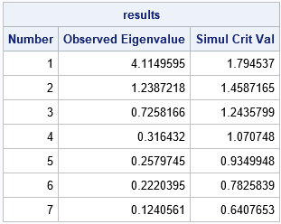
The table is qualitatively the same as the one produced by PROC FACTOR. Both tables are the results of simulations, so you should expect to see small differences in the third column, which shows the 95th percentile of the distributions of the eigenvalues.

Visualize the distribution of eigenvalues

The eigenvalues are stored as rows of the simEigen matrix, so you can estimate the 5th, 10th, ..., 95th percentiles and over band plots on the eigenvalue (scree) plot, as follows:

/* 4. Create a graph that illustrates Horn's method: 
   Factor Number vs distribution of eigenvalues. Write results in long form. */
/* 4a. Write the observed eigenvalues and the 95th percentile */
create Horn from results[c={"Factor" "Eigenvalue" "SimulCritVal"}];
   append from results;
close;
 
/* 4b. Visualize the uncertainty in the simulated eigenvalues. For details, see
   https://blogs.sas.com/content/iml/2020/10/12/visualize-uncertainty-regression-predictions.html 
*/
a = do(0.05, 0.45, 0.05);          /* significance levels */
call qntl(Lower, simEigen, a);     /* lower qntls         */
call qntl(Upper, simEigen, 1-a);   /* upper qntls         */
Factor = col(Lower);               /* 1,2,3,...,1,2,3,... */
alpha = repeat(a`, 1, p);             
create EigenQntls var {"Factor" "alpha" "Lower" "Upper"};
   append;
close;
QUIT;
 
proc sort data=EigenQntls;
   by alpha Factor;
run;
data All;
   set Horn EigenQntls;
run;
 
title "Horn's Method (1965) for Choosing the Number of Factors";
title2 "Also called Parallel Analysis";
proc sgplot data=All noautolegend;
   band x=Factor lower=Lower upper=Upper/ group=alpha fillattrs=(color=gray) transparency=0.9;
   series x=Factor y=Eigenvalue / markers name='Eigen' legendlabel='Observed Eigenvalue';
   series x=Factor y=SimulCritVal / markers lineattrs=(pattern=dot) 
          name='Sim' legendlabel='Simulated Crit Value';
   keylegend 'Eigen' 'Sim' / across=1;
run;

The graph is shown in the previous section. The darkest part of the band shows the median eigenvalue. You can see that the "null distribution" of eigenvalues is rather narrow, even though the data contain only 50 observations. I thought perhaps it would be wider. Because the band is narrow, it doesn't matter much whether you choose the 95th percentile as a critical value or some other value (90th percentile, 80th percentile, and so forth). For these data, any reasonable choice for a percentile will still lead to rejecting the second factor and keeping only one principal component. Because the band is narrow, the results will not be unduly affected by whether you use few or many Monte Carlo simulations. In this article, both simulations used B=1000 simulations.

Summary

In summary, PROC FACTOR supports the PARALLEL and PLOTS=PARALLEL options for performing a "parallel analysis," which is Horn's method for choosing the number of principal components to retain. PROC FACTOR creates a table and graph that summarize Horn's method. You can also run the simulation yourself. If you use SAS/IML, you can simulate the correlation matrices directly, which is more efficient than simulating the data. If you run the simulation yourself, you can add additional features to the scree plot, such as a confidence band that shows the null distribution of the eigenvalues.

Blogs