The expected value of the tail of a distribution

The expected value of a random variable is essentially a weighted mean over all possible values. You can compute it by summing (or integrating) a probability-weighted quantity over all possible values of the random variable. The expected value is a measure of the "center" of a probability distribution.

Expected value for the tail of a distribution

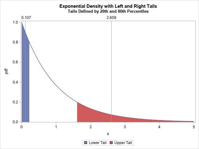
You can generalize this idea. Instead of using the entire distribution, suppose you want to find the "center" of only a portion of the distribution. For the central portion of a distribution, this process is similar to the trimmed mean. (The trimmed mean discards data in the tails of a distribution and averages the remaining values.) For the tails of a distribution, a natural way to compute the expected value is to sum (or integrate) the weighted quantity x*pdf(x) over the tail of the distribution. The graph to the right illustrates this idea for the exponential distribution. The left and right tails (defined by the 20th and 80th percentiles, respectively) are shaded and the expected value in each tail is shown by using a vertical reference line.

This article shows how to compute the expected value of the tail of a probability distribution. It also shows how to estimate this quantity for a data sample.

Why is this important? Well, this idea appears in some papers about robust and unbiased estimates of the skewness and kurtosis of a distribution (Hogg, 1974; Bono, et al., 2020). In estimating skewness and kurtosis, it is important to estimate the length of the tails of a distribution. Because the tails of many distributions are infinite in length, you need some alternative definition of "tail length" that leads to finite quantities. One approach is to truncate the tails, such as at the 5th percentile on the left and the 95th percentile on the right. An alternative approach is to use the expected value of the tails, as shown in this article.

The expected value in a tail

Suppose you have any distribution with density function f. You can define the tail distribution as a truncated distribution on the interval (a,b), where possibly a = -∞ or b = ∞. To get a proper density, you need to divide by the area of the tail, as follows:
$g(x) = f(x) / \int_a^b f(x) \,dx$
If F(x) is the cumulative distribution, the denominator is simply the expression F(b) – F(a). Therefore, the expected value for the truncated distribution on (a,b) is
$EV = \int_a^b x g(x) \,dx = (\int_a^b x f(x) \,dx) / (F(b) - F(a))$

There is no standard definition for the "tail" of a distribution, but one definition is to use symmetric quantiles of the distribution to define the tails. For a quantile, p, you can define the left tail to be the portion of the distribution for which X ≤ p and the right tail to be the portion for which X ≥ 1-p. If you let q_L be the pth quantile and q_U be the (1-p)th quantile, then the expected value of the left tail is
$E_L = (\int_{-\infty}^{q_L} x f(x) \,dx) / (F(q_L) - 0)$
and the expected value of the right tail is
$E_R = (\int_{q_U}^{\infty} x f(x) \,dx) / (1 - F(q_U))$

The expected value in the tail of the exponential distribution

For an example, let's look at the exponential distribution. The exponential distribution is defined only for x ≥ 0, so the left tail starts a 0. The choice of the quantile, p, is arbitrary, but I will use p=0.2 because that value is used in Bono, et al. (2020). The 20th percentile of the exponential distribution is q20 = 0.22. The 80th percentile is q80 = 1.61. You can use the QUAD function in the SAS/IML language to compute the integrals, as follows:

proc iml;
/* find the expected value of the truncated exponential distribution on the interval [a,b] 
*/
start Integrand(x);
   return x*pdf("Expon",x);
finish;
 
/* if f(x) is the PDF and F(x) is the CDF of a distribution, the expected value on [a,b] is
   (\int_a^b  x*f(x) dx) / (CDF(B) - CDF(a))
*/
start Expo1Moment(a,b);
   call quad(numer, "Integrand", a||b );
   /* define CDF(.M)=0 and CDF(.P)=1 */
   cdf_a = choose(a=., 0, cdf("Expon", a));  /* CDF(a) */
   cdf_b = choose(b=., 1, cdf("Expon", b));  /* CDF(b) */
   ExpectedValue = numer / (cdf_b - cdf_a);
   return ExpectedValue;
finish;
 
/* expected value of lower 20th percentile of Expon distribution */
p = 0.2;
qLow = quantile("Expon", p);
ExpValLow20 = Expo1Moment(0, qLow);
print qLow ExpValLow20;
 
/* expected value of upper 20th percentile */
qHi = quantile("Expon", 1-p);
ExpValUp20 = Expo1Moment(qHi, .I); /* .I = infinity */
print qHi ExpValUp20;

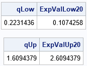
In this program, the left tail is the portion of the distribution to the left of the 20th percentile. The right tail is to the right of the 80th percentile. The first table says that the expected value in the left tail of the exponential distribution is 0.107. Intuitively, that is the weighted average of the left tail or the location of its center of mass. The second table says that the expected value in the right tail is 2.609. These results are visualized in the graph at the top of this article.

Estimate the expected value in the tail of a distribution

You can perform a similar computation for a data sample. Instead of an integral, you merely take the average of the lower and upper p*100% of the data. For example, the following SAS/IML statements simulate 100,000 random variates from the exponential distribution. You can use the QNTL function to estimate the quantiles of the data. You can then use the LOC function to find the elements that are in the tail and use the MEAN function to compute the arithmetic average of those elements:

/* generate data from the exponential distribution */
call randseed(12345);
N = 1e5;
x = randfun(N, "Expon");
 
/* assuming no duplicates and a large sample, you can 
   use quantiles and means to estimate the expected values */
/* estimate the expected value for the lower 20% tail */
call qntl(qEst, x, p);      /* p_th quantile */
idx = loc(x<=qEst);         /* rows for which x[i]<= quantile */
meanLow20 = mean(x[idx]);   /* mean of lower tail */
print qEst meanLow20;
 
/* estimate the expected value for the upper 20% tail */
call qntl(qEst, x, 1-p);    /* (1-p)_th quantile */
idx = loc(x>=qEst);         /* rows for which x[i]>= quantile */
meanUp20 = mean(x[idx]);    /* mean of upper tail */
print qEst meanUp20;

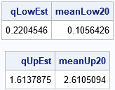
The estimates are shown for the lower and upper 20th-percentile tails of the data. Because the sample is large, the sample estimates are close to the quantiles of the exponential distribution. Also, the means of the lower and upper tails of the data are close to the expected values for the tails of the distribution.

It is worth mentioning that there are many different formulas for estimating quantiles. Each estimator will give a slightly different estimate for quantile, and therefore you can get different estimates for the mean. This becomes important for small samples, for long-tailed distributions, and for samples that have duplicate values.

Summary

The expected value is a measure of the "center" of a probability distribution on some domain. This article shows how to solve an integral to find the expected value for the left tail or right tail of a distribution. For a data distribution, the expected value is the mean of the observations in the tail. In a future article, I'll show how to use these ideas to create robust and unbiased estimates of skewness and kurtosis.

Blogs