In last week's article about the Flint water crisis, I computed the 90th percentile of a small data set. Although I didn't mention it, the value that I reported is different from the the 90th percentile that is reported in Significance magazine.

That is not unusual. The data only had 20 unique values, and there are many different formulas that you can use to compute sample percentiles (generally called quantiles). Because different software packages use different default formulas for sample quantiles, it is not uncommon for researchers to report different quantiles for small data sets. This article discusses the five percentile definitions that are supported in SAS software.

You might wonder why there are multiple definitions. Recall that a sample quantile is an estimate of a population quantile. Statisticians have proposed many quantile estimators, some of which are based on the empirical cumulative distribution (ECDF) of the sample, which approximates the cumulative distribution function (CDF) for the population. The ECDF is a step function that has a jump discontinuity at each unique data value. Consequently, the inverse ECDF does not exist and the quantiles are not uniquely defined.

Definitions of sample quantiles

In SAS, you can use the PCTLDEF= option in PROC UNIVARIATE or the QNTLDEF= option in other procedures to control the method used to estimate quantiles. A sample quantile does not have to be an observed data value because you are trying to estimate an unknown population parameter.

For convenience, assume that the sample data are listed in sorted order. In high school, you probably learned that if a sorted sample has an even number of observations, then the median value is the average of the middle observations. The default quantile definition in SAS (QNTLDEF=5) extends this familiar rule to other quantiles. Specifically, if the sample size is N and you ask for the q_th quantile, then when Nq is an integer, the quantile is the data value x[Nq]. However, when Nq is not an integer, then the quantile is defined (somewhat arbitrarily) as the average of the two data x[j] and x[j+1], where j = floor(Nq). For example, if N=10 and you want the q=0.17 quantile, then Nq=1.7, so j=1 and the 17th percentile is reported as the midpoint between the ordered values x[1] and x[2].

Averaging is not the only choices you can make when Nq is not an integer. The other percentile definitions correspond to making different choices. For example, you could round Nq down (QNTLDEF=3), or you could round it to the nearest integer (QNTLDEF=2). Or you could use linear interpolation (QNTLDEF=1 and QNTLDEF=4) between the data values whose (sorted) indices are closest to Nq. In the example where N=10 and q=0.17, the QNTLDEF=1 interpolated quantile is 0.3 x[1] + 0.7 x[2].

Visualizing the definitions for quantiles

The SAS documentation contains the formulas used for the five percentile definitions, but sometimes a visual comparison is easier than slogging through mathematical equations. The differences between the definitions are most apparent on small data sets that contain integer values, so let's create a tiny data set and apply the five definitions to it. The following example has 10 observations and six unique values.

data Q;
input x @@;
datalines;
0 1 1 1 2 2 2 4 5 8
;

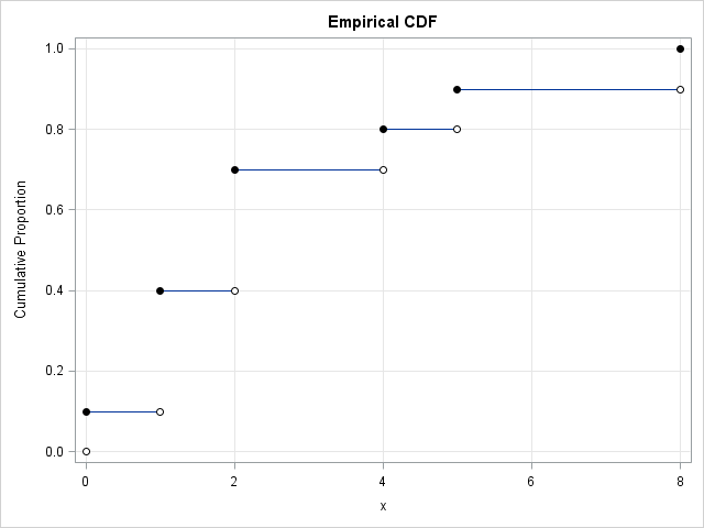
You can use PROC UNIVARIATE or other methods to plot the empirical cumulative proportions, as shown. Because the ECDF is a step function, most cumulative proportions values (such as 0.45) are "in a gap." By this I mean that there is no observation t in the data for which the cumulative proportion P(X ≤ t) equals 0.45. Depending on how you define the sample quantiles, the 0.45 quantile might be reported as 1, 1.5, 1.95, or 2.

Since the default definition is QNTLDEF=5, let's visualize the sample quantiles for that definition. You can use the PCTPTS= option on the OUTPUT statement in PROC UNIVARIATE to declare the percentiles that you want to compute. Equivalently, you can use the QNTL function in PROC IML, as below. Regardless, you can ask SAS to find the quantiles for a set of probabilities on a fine grid of points such as {0.001, 0.002, ..., 0.998, 0.999}. You can the graph of the probabilities versus the quantiles to visualize how the percentile definition computes quantiles for the sample data.

proc iml;
use Q; read all var "x"; close;       /* read data */
prob = T(1:999) / 1000;               /* fine grid of prob values */
call qntl(quantile, x, prob, 5);      /* use method=5 definition  */
create Pctls var {"quantile" "prob" "x"}; append; close;
quit;
 
title "Sample Percentiles";
title2 "QNTLDEF = 5";
proc sgplot data=Pctls noautolegend;
   scatter x=quantile y=prob / markerattrs=(size=5 symbol=CircleFilled);
   fringe x / lineattrs=GraphData2(thickness=3);
   xaxis display=(nolabel) values=(0 to 8);
   yaxis offsetmin=0.05 grid values=(0 to 1 by 0.1) label="Cumulative Proportions";
   refline 0 1 / axis=y;
run;

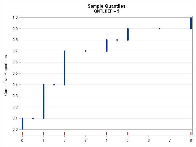
For each probability value (Y axis), the graph shows the corresponding sample quantile (X axis) for the default definition in SAS, which is QNTLDEF=5. The X axis also displays red tick marks at the location of the data. You can use this graph to find any quantile. For example, to find the 0.45 quantile, you start at 0.45 on the Y axis, move to the right until you hit a blue marker, and then drop down to the X axis to discover that the 0.45 quantile estimate is 2.

If you prefer to think of the quantiles (the X values) as a function of the probabilities, just interchange the X= and Y= arguments in the SCATTER statement (or turn your head sideways!). Then the quantile function is a step function.

Comparing all five SAS percentile definitions

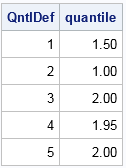
It is easy to put a loop around the SAS/IML computation to compute the sample quantiles for the five different definitions that are supported in SAS. The following SAS/IML program writes a data set that contains the sample quantiles. You can use the WHERE statement in PROC PRINT to compare the same quantile across the different definitions. For example, the following displays the 0.45 quantile (45th percentile) for the five definitions:

/* Compare all SAS methods */
proc iml;
use Q; read all var "x"; close;       /* read data */
prob = T(1:999) / 1000;               /* fine grid of prob values */
create Pctls var {"Qntldef" "quantile" "prob" "x"};
do def = 1 to 5;
   call qntl(quantile, x, prob, def); /* qntldef=1,2,3,4,5 */
   Qntldef = j(nrow(prob), 1, def);   /* ID variable */
   append;
end;
close;
quit;
 
proc print data=Pctls noobs;
   where prob = 0.45;                 /* compare 0.45 quantile for different definitions */
   var Qntldef quantile;
run;

You can see that the different definitions lead to different sample quantiles. How do the quantile functions compare? Let's plot them and see:

ods graphics / antialiasmax=10000;
title "Sample Percentiles in SAS";
proc sgpanel data=Pctls noautolegend;
   panelby Qntldef / onepanel rows=2;
   scatter x=quantile y=prob/ markerattrs=(size=3 symbol=CircleFilled);
   fringe x;
   rowaxis offsetmax=0 offsetmin=0.05 grid values=(0 to 1 by 0.1) label="Cumulative Proportion";
   refline 0 1 / axis=y;
   colaxis display=(nolabel);
run;

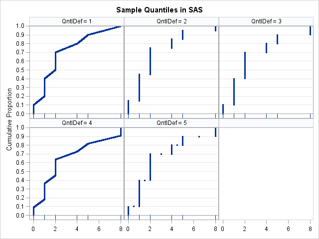
The graphs (click to enlarge) show that QNTLDEF=1 and QNTLDEF=4 are piecewise-linear interpolation methods, whereas QNTLDEF=2, 3, and 5 are discrete rounding methods. The default method (QNTLDEF=5) is similar to QNTLDEF=2 except for certain averaged values. For the discrete definitions, SAS returns either a data value or the average of adjacent data values. The interpolation methods do not have that property: the methods will return quantile values that can be any value between observed data values.

If you have a small data set, as in this blog post, it is easy to see how the percentile definitions are different. For larger data sets (say, 100 or more unique values), the five quantile functions look quite similar.

The differences between definitions are most apparent when there are large gaps between adjacent data values. For example, the sample data has a large gap between the ninth and tenth observations, which have the values 5 and 8, respectively. If you compute the 0.901 quantile, you will discover that the "round down" method (QNTLDEF=2) gives 5 as the sample quantile, whereas the "round up" method (QNTLDEF=3) gives the value 8. Similarly, the "backward interpolation method" (QNTLDEF=1) gives 5.03, whereas the "forward interpolation method" (QNTLDEF=4) gives 7.733.

In summary, this article shows how the (somewhat obscure) QNTLDEF= option results in different quantile estimates. Most people just accept the default definition (QNTLDEF=5), but if you are looking for a method that interpolates between data values, rather than a method that rounds and averages, I recommend QNTLDEF=1, which performs linear interpolations of the ECDF. The differences between the definitions are most apparent for small samples and when there are large gaps between adjacent data values.

To learn about how quantile estimates are defined in other software packages, see "Sample quantiles: A comparison of 9 definitions."

Reference

For more information about sample quantiles, including a mathematical discussion of the various formulas, see
Hyndman, R. J. and Fan, Y. (1996) "Sample quantiles in statistical packages", American Statistician, 50, 361–365.