According to Hyndman and Fan ("Sample Quantiles in Statistical Packages," TAS, 1996), there are nine definitions of sample quantiles that commonly appear in statistical software packages. Hyndman and Fan identify three definitions that are based on rounding and six methods that are based on linear interpolation. This blog post shows how to use SAS to visualize and compare the nine common definitions of sample quantiles. It also compares the default definitions of sample quantiles in SAS and R.

Definitions of sample quantiles

Suppose that a sample has N observations that are sorted so that x[1] ≤ x[2] ≤ ... ≤ x[N], and suppose that you are interested in estimating the p_th quantile (0 ≤ p ≤ 1) for the population. Intuitively, the data values near x[j], where j = floor(Np) are reasonable values to use to estimate the quantile. For example, if N=10 and you want to estimate the quantile for p=0.64, then j = floor(Np) = 6, so you can use the sixth ordered value (x[6]) and maybe other nearby values to estimate the quantile.

Hyndman and Fan (henceforth H&F) note that the quantile definitions in statistical software have three properties in common:

• The value p and the sample size N are used to determine two adjacent data values, x[j]and x[j+1]. The quantile estimate will be in the closed interval between those data points. For the previous example, the quantile estimate would be in the closed interval between x[6] and x[7].
• For many methods, a fractional quantity is used to determine an interpolation parameter, λ. For the previous example, the fraction quantity is (Np - j) = (6.4 - 6) = 0.4. If you use λ = 0.4, then an estimate the 64th percentile would be the value 40% of the way between x[6] and x[7].
• Each definition has a parameter m, 0 ≤ m ≤ 1, which determines how the method interpolates between adjacent data points. In general, the methods define the index j by using j = floor(Np + m). The previous example used m=0, but other choices include m=0.5 or values of m that depend on p.

Thus a general formula for quantile estimates is q = (1 - λ) x[j]+ λ x[j+1], where λ and j depend on the values of p, N, and a method-specific parameter m.

You can read Hyndman and Fan (1986) for details or see the Wikipedia article about quantiles for a summary. The Wikipedia article points out a practical consideration: for values of p that are very close to 0 or 1, some definitions need to be slightly modified. For example, if p < 1/N, the quantity Np < 1 and so j = floor(Np) equals 0, which is an invalid index. The convention is to return x[1] when p is very small and return x[N] when p is very close to 1.

Compute all nine sample quantile definitions in SAS

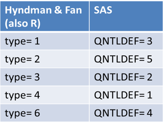
SAS has built-in support for five of the quantile definitions, notably in PROC UNIVARIATE, PROC MEANS, and in the QNTL subroutine in SAS/IML. You can use the QNTLDEF= option to choose from the five definitions. The following table associates the five QNTLDEF= definitions in SAS to the corresponding definitions from H&F, which are also used by R. In R you choose the definition by using the type parameter in the quantile function.

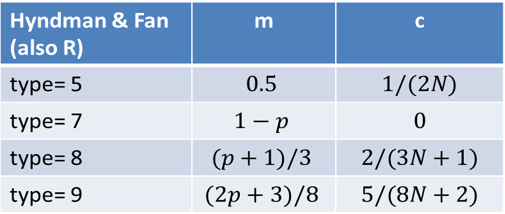
It is straightforward to write a SAS/IML function to compute the other four definitions in H&F. In fact, H&F present the quantile interpolation functions as specific instances of one general formula that contains a parameter, which they call m. As mentioned above, you can also define a small value c (which depends on the method) such that the method returns x[1] if p < c, and the method returns x[N] if p ≥ 1 - c.

The following table presents the parameters for computing the four sample quantile definitions that are not natively supported in SAS:

Visualizing the definitions of sample quantiles

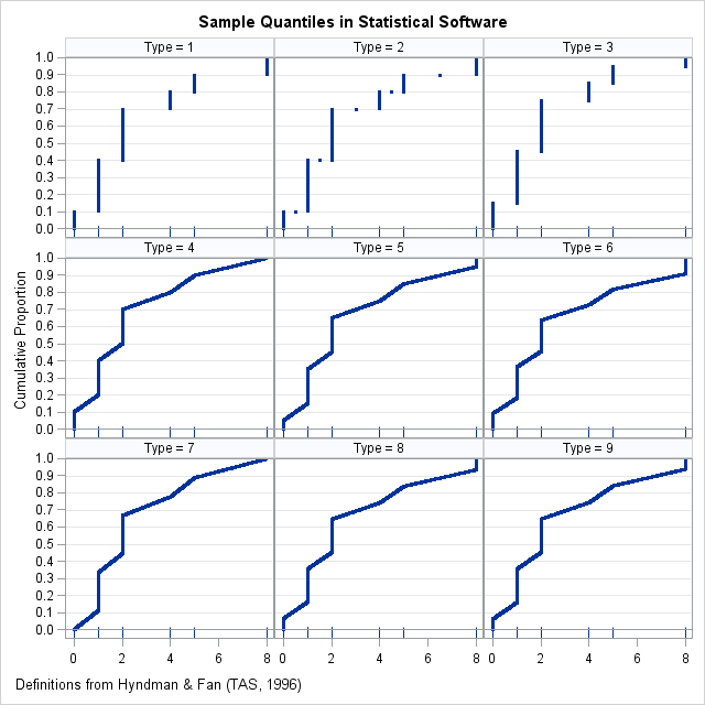
You can download the SAS program that shows how to compute sample quantiles and graphs for any of the nine definitions in H&F. The differences between the definitions are most evident for small data sets and when there is a large "gap" between one or more adjacent data values. The following panel of graphs shows the nine sample quantile methods for a data set that has 10 observations, {0 1 1 1 2 2 2 4 5 8}. Each cell in the panel shows the quantiles for p = 0.001, 0.002, ..., 0.999. The bottom of each cell is a fringe plot that shows the six unique data values.

In these graphs, the horizontal axis represents the data and quantiles. For any value of x, the graph estimates the cumulative proportion of the population that is less than or equal to x. Notice that if you turn your head sideways, you can see the quantile function, which is the inverse function that estimates the quantile for each value of the cumulative probability.

You can see that although the nine quantile functions have the same basic shape, the first three methods estimate quantiles by using a discrete rounding scheme, whereas the other methods use a continuous interpolation scheme.

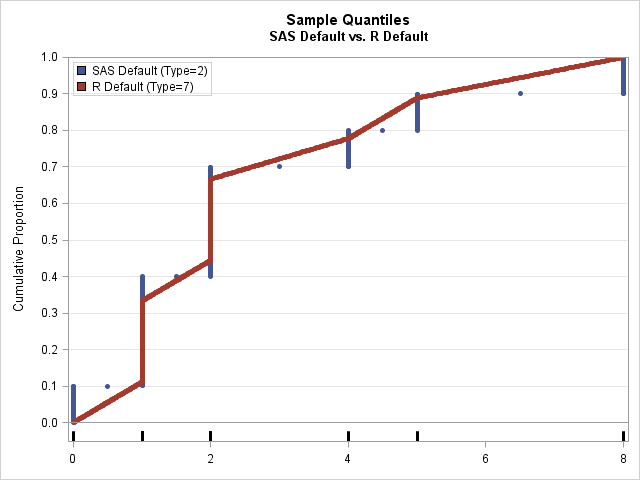
You can use the same data to compare methods. Instead of plotting each quantile definition in its own cell, you can overlay two or more methods. For example, by default, SAS computes sample quantiles by using the type=2 method, whereas R uses type=7 by default. The following graph overlays the sample quantiles to compare the default methods in SAS and R on this tiny data set. The default method in SAS always returns a data value or the average of adjacent data values; the default method in R can return any value in the range of the data.

Does the definition of sample quantiles matter?

As shown above, different software packages use different defaults for sample quantiles. Consequently, when you report quantiles for a small data set, it is important to report how the quantiles were computed.

However, in practice analysts don't worry too much about which definition they are using because the difference between methods is typically small for larger data sets (100 or more observations). The biggest differences are often between the discrete methods, which always report a data value or the average between two adjacent data values, and the interpolation methods, which can return any value in the range of the data. Extreme quantiles can also differ between the methods because the tails of the data often have fewer observations and wider gaps.

The following graph shows the sample quantiles for 100 observations that were generated from a random uniform distribution. As before, the two sample quantiles are type=2 (the SAS default) and type=7 (the R default). At this scale, you can barely detect any differences between the estimates. The red dots (type=7) are on top of the corresponding blue dots (type=2), so few blue dots are visible.

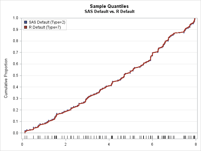
So does the definition of the sample quantile matter? Yes and no. Theoretically, the different methods compute different estimates and have different properties. If you want to use an estimator that is unbiased or one that is based on distribution-free computations, feel free to read Hyndman and Fan and choose the definition that suits your needs. The differences are evident for tiny data sets. On the other hand, the previous graph shows that there is little difference between the methods for moderately sized samples and for quantiles that are not near gaps. In practice, most data analysts just accept the default method for whichever software they are using.

In closing, I will mention that there are other quantile estimation methods that are not simple formulas. In SAS, the QUANTREG procedure solves a minimization problem to estimate the quantiles. The QUANTREG procedure enables you to not only estimate quantiles, but also estimate confidence intervals, weighted quantiles, the difference between quantiles, conditional quantiles, and more.

SAS program to compute nine sample quantiles.