A SAS programmer recently asked why his SAS program and his colleague's R program display different estimates for the quantiles of a very small data set (less than 10 observations). I pointed the programmer to my article that compares the nine common definitions for sample quantiles. The article has a section that explicitly compares the default sample quantiles in SAS and R. The function in the article is written to support all nine definitions. The programmer asked whether I could provide a simpler function that computes only the default definition in R.

This article compares the default sample quantiles in SAS in R. It is a misnomer to refer to one definition as "the SAS method" and to another as "the R method." In SAS, you can use the PCTLDEF= option in PROC UNIVARIATE or the QNTLDEF= option in other procedures to use one of five different quantile estimates. By using SAS/IML, you can compute all nine estimation methods. Similarly, R supports all nine definitions. However, users of statistical software often use the default methods, then wonder why they get different answers from different software. This article explains the difference between the DEFAULT method in SAS and the DEFAULT method in R. The default in R is also the default method in Julia and in the Python packages SciPy and NumPy.

The Hyndman and Fan taxonomy

The purpose of a sample statistic is to estimate the corresponding population parameter. That is, the sample quantiles are data-based estimates of the unknown quantiles in the population. Hyndman and Fan ("Sample Quantiles in Statistical Packages," TAS, 1996), discuss nine definitions of sample quantiles that commonly appear in statistical software packages. All nine definitions result in valid estimates. For large data sets (say, 100 or more observations), they tend to give similar results. The differences between the definitions are most evident if you use a small data set that has wide gaps between two adjacent pairs of values (after sorting the data). The example in this article is small and has a wide gap between the largest value and the next largest value.

By default, SAS uses Hyndman and Fan's Type=2 method, whereas R (and Julia, SciPy, and NumPy) use the Type=7 method. The Type=2 method uses the empirical cumulative distribution of the data (empirical CDF) to estimate the quantiles, whereas the Type=7 method uses a piecewise-linear estimate of the cumulative distribution function. This is demonstrated in the next section.

An example of sample quantiles

To focus the discussion, consider the data {0, 1, 1, 1, 2, 2, 2, 4, 5, 8}. There are 10 observations, but only six unique values. The following graphs show the estimates of the cumulative distribution function used by the Type=2 and Type=7 methods. The fringe plot (rug plot) below the CDF shows the locations of the data:

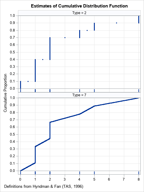
The sample quantiles are determined by the estimates of the CDF. The largest gap in the data is between the values X=5 and X=8. So, for extreme quantiles (greater than 0.9), we expect to see differences between the Type=2 and the Type=7 estimates for extreme quantiles. The following examples show that the two methods agree for some quantiles, but not for others:

• The 0.5 quantile (the median) is determined by drawing a horizontal line at Y=0.5 and seeing where the horizontal line crosses the estimate of the CDF. For both graphs, the corresponding X value is X=2, which means that both methods give the same estimate (2) for the median.
• The 0.75 quantile (the 75th percentile) estimates are different between the two methods. In the upper graph, a horizontal line at 0.75 crosses the empirical CDF at X=4, which is a data value. In the lower graph, the estimate for the 0.75 quantile is X=3.5, which is neither a data value nor the average of adjacent values.
• The 0.95 quantile (the 95th percentile) estimates are different. In the upper graph, a horizontal line at 0.95 crosses the empirical CDF at X=8, which is the maximum data value. In the lower graph, the estimate for the 0.95 quantile is X=6.65, which is between the two largest data values.

Comments on the CDF estimates

The Type=2 method (the default in SAS) uses an empirical CDF (ECDF) to estimate the population quantiles. The ECDF has a long history of being used for fitting and comparing distributions. For example, the Kolmogorov-Smirnov test uses the ECDF to compute nonparametric goodness-of-fit tests. When you use the ECDF, a quantile is always an observed data value or the average of two adjacent data values.

The Type=7 method (the default in R) uses a piecewise-linear estimate to the CDF. There are many ways to create a piecewise-linear estimate, and there have been many papers (going back to the 1930's) written about the advantages and disadvantages of each choice. In Hyndman and Fan's taxonomy, six of the nine methods use piecewise-linear estimates. Some people prefer the piecewise-linear estimates because the inverse CDF is continuous: a small change to the probability value (such as 0.9 to 0.91) results in a small change to the quantile estimates. This is property is not present in the methods that use the ECDF.

A function to compute the default sample quantiles in R

Back in 2017, I wrote a SAS/IML function that can compute all of the common definitions of sample quantiles. If you only want to compute the default (Type=7) definition in R, you can use the following simpler function:

proc iml;
/* By default, R (and Julia, and some Python packages) uses
   Hyndman and Fan's Type=7 definition. Compute Type=7 sample quantiles.
*/
start GetQuantile7(y, probs);
   x = colvec(y);
   N = nrow(x);
   if N=1 then return (y);  /* handle the degenerate case, N=1 */
 
   /* remove missing values, if any */
   idx = loc(x^=.);
   if ncol(idx)=0 then  
      return (.);           /* all values are missing */
   else if ncol(idx)<N then do;
      x = x[idx,]; N = nrow(x);  /* remove missing */
   end;
 
   /* Main computation: Compute Type=7 sample quantile. 
      Estimate is a linear interpolation between x[j] and x[j+1]. */
   call sort(x);
   p = colvec(probs);
   m = 1-p;
   j = floor(N*p + m);      /* indices into sorted data values */
   g = N*p + m - j;         /* 0 <= g <= 1 for interpolation */
 
   q = j(nrow(p), 1, x[N]); /* if p=1, estimate by x[N]=max(x) */
   idx = loc(p < 1);
   if ncol(idx) >0 then do;
      j = j[idx]; g = g[idx];
      q[idx] = (1-g)#x[j] + g#x[j+1]; /* linear interpolation */
   end;   
   return q;
finish;
 
/* Compare the SAS and R default definitions.
   The differences between definitions are most apparent 
   for small samples that have large gaps between adjacent data values. */
x = {0 1 1 1 2 2 2 4 5 8}`;
prob = {0.5, 0.75, 0.9, 0.95};
 
call qntl(SASDefaultQntl, x, prob);
RDefaultQntl = GetQuantile7(x, prob);
print prob SASDefaultQntl RDefaultQntl;

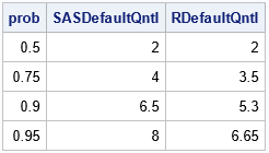
The table shows some of the quantiles that were discussed previously. If you choose prob to be evenly spaced points in [0,1], you get the values on the graphs shown previously.

Summary

There are many ways to estimate quantiles. Hyndman and Fan (1996) list nine common definitions. By default, SAS uses the Type=2 method, where R (and other software) uses the Type=7 method. SAS procedures support five of the nine common definitions of sample quantiles, and you can use SAS/IML to compute the remaining definitions. To make it easy to reproduce the default values of sample quantiles from other software, I have written a SAS/IML function that computes the Type=7 quantiles.

If you do not have SAS/IML software, but you want to compute estimates that are based on a piecewise-linear estimate of the CDF, I suggest you use the PCTLDEF=1 option in PROC UNIVARIATE (or QNTLDEF=1 in PROC MEANS). This produces the Type=4 method in Hyndman and Fan's taxonomy. For more information about the quantile definitions that are natively available in SAS procedures, see "Quantile definitions in SAS."