The April 2017 issue of Significance magazine features a cover story by Robert Langkjaer-Bain about the Flint (Michigan) water crisis. For those who don't know, the Flint water crisis started in 2014 when the impoverished city began using the Flint River as a source of city water. The water was not properly treated, which led to unhealthy (even toxic) levels of lead and other contaminants in the city's water supply. You can read an overview of the Flint Water Crisis on Wikipedia.

The crisis was compounded because someone excluded two data points before computing a quantile of a small data set. This seemingly small transgression had tragic ramifications. This blog post examines the Flint water quality data and shows why excluding those two points changed the way that the city responded. You can download the SAS program that analyzes these data.

Federal standards for detecting unsafe levels of lead

The federal Lead and Copper Rule of 1991 specifies a statistical method for determining when the concentration of lead in a water supply is too high. First, you sample from a number of "worst case" homes (such as those served by lead pipes), then compute the 90th percentile of the lead levels from those homes. If the 90th percentile exceeds 15 parts per billion (ppb), then the water is unsafe and action must be taken to correct the problem.

In spring 2015, this data collection and analysis was carried out in Flint by the Michigan Department of Environmental Quality (MDEQ), but according to the Significance article, the collection process was flawed. For example, the MDEQ was supposed to collect 100 measurements, but only 71 samples were obtained, and they were not from the "worst case" homes. The 71 lead measurements that they collected are reproduced below, where I have used '0' for "not detectable." A call to PROC MEANS computes the 90th percentile (P90) of the complete sample:

/* values of lead concentration in Flint water samples.
   Use 0 for "not detectable" */
data FlintObs;
label Lead = "Lead Concentration (ppb)";
input lead @@;
Exclude = (Lead=20 | Lead=104); /* MDEQ excluded these two large values */
datalines;
0 0 0 0 0 0 0 0 0 0 0 0 0 
1 1 1 1 2 2 2 2 2 2 2 2 2 2 2 
3 3 3 3 3 3 3 3 3 3 3 4 4 
5 5 5 5 5 5 5 5 6 6 6 6 7 7 7 
8 8 9 10 10 11 13 18 20 21 22 29 43 43 104
;
 
proc means data=FlintObs N p90; 
   var lead;
run;

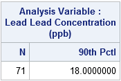
In this analysis of the full data, the 90th percentile of the sample is 18 ppb, which exceeds the federal limit of 15 ppb. Consequently, the Flint water fails the safety test, and the city must take action to improve the water.

But that is not what happened. Allegedly, "the MDEQ told the city's water quality supervisors to remove two of the samples" (Langkjaer-Bain, p. 19) that were over 15 ppb. The MDEQ claimed that these data were improperly collected. The two data points that were excluded have the values 20 and 104. Because these values are both higher than the 90th percentile, excluding these observations lowered the 90th percentile of the modified sample, which has 69 observations. The following call to PROC MEANS computes the 90th percentile for the modified sample:

proc means data=FlintObs N p90; 
   where Exclude=0;     /* exclude two observations */
   var lead;
run;

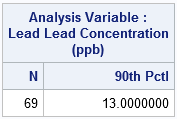
The second table shows that the 90th percentile of the modified sample is 13 ppb. "The exclusion of these two samples nudged the 90th percentile reading...below the all-important limit of 15 ppb." (Langkjaer-Bain, p. 20) The modified conclusion is that the city does not need to undertake expensive corrective action to render the water safe.

The following histogram (click to enlarge) is similar to Figure 1 in Langkjaer-Bain's article. The red bars indicate observations that the MDEQ excluded from the analysis. The graph clearly shows that the distribution of lead values has a long tail. A broken axis is used to indicate that the distance to the 104 ppb reading has been shortened to reduce horizontal space. The huge gap near 15 ppb indicates a lack of data near that important value. Therefore the quantiles near that point will be extremely sensitive to deleting extreme values. To me, the graph indicates that more data should be collected so that policy makers can be more confident in their conclusions.

Confidence intervals for the 90th percentile

Clearly the point estimate for the 90th percentile depends on whether or not those two measurements are excluded. But can statistics provide any additional insight into the 90th percentile of lead levels in the Flint water supply? When someone reports a statistic for a small sample, I like to ask "how confident are you in that statistic?" A standard error is one way to express the accuracy of a point estimate; a 95% confidence interval (CI) is another. The width of a confidence interval gives us information about the accuracy of the point estimate. As you might expect, the standard error for an extreme quantile (such as 0.9) is typically much bigger than for a quantile near 0.5, especially when there isn't much data near the quantile.

Let's use SAS procedures to construct a 95% CI for the 90th percentile. PROC UNIVARIATE supports the CIPCTLDF option, which produces distribution-free confidence intervals. I'll give the Flint officials the benefit of the doubt and compute a confidence interval for the modified data that excluded the two "outliers":

proc univariate data=FlintObs CIPctlDF;
   where Exclude=0;     /* exclude two observations */
   var Lead;
   ods select quantiles;
run;

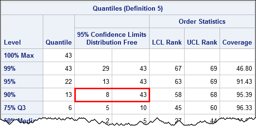
The 95% confidence interval for P90 is [8, 43], which is very wide and includes the critical value 15 ppb in its interior. If someone asks, "how confident are you that the 90th percentile does not exceed 15 ppb," you should respond, "based on these data, I am not confident at all."

Statistical tests for the 90th percentile

As I've written before, you can also use the QUANTREG procedure in SAS to provide an alternative method to compute confidence intervals for percentiles. Furthermore, the QUANTREG procedure supports the ESTIMATE statement, which you can use to perform a one-sided test for the hypothesis "does the 90th percentile exceed 15 ppb?" The following call to PROC QUANTREG performs this analysis and uses 10,000 bootstrap resamples to estimate the confidence interval:

proc quantreg data=FlintObs CI=resampling(nrep=10000);
   where Exclude=0;     /* exclude two observations */
   model lead = / quantile=0.9 seed=12345;
   estimate 'P90 > 15' Intercept 1 / upper CL testvalue=15;
   ods select ParameterEstimates Estimates;
run;

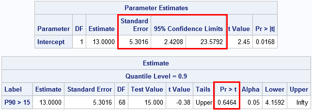
The standard error for the 90th percentile is about 5.3. Based on bootstrap resampling methods, the 95% CI for P90 is approximately [2.4, 23.6]. (Other methods for estimating the CI give similar or wider intervals.) The ESTIMATE statement is used to test the null hypothesis that P90 is greater than 15. The p-value is large, which means that even if you delete two large lead measurements, the data do not provide evidence to reject the null hypothesis.

Conclusions

There is not enough evidence to reject the hypothesis that P90 is greater than the legal limit of 15 ppb. Two different 95% confidence intervals for P90 include 15 ppb in their interiors.

In fact, the confidence intervals include 15 ppb whether you use all 71 observations or just the 69 observations that MDEQ used. So you can argue about whether the MDEQ should have excluded the controversial measurements, but the hypothesis test gives the same conclusion regardless. By using these data, you cannot rule out the possibility that the 90th percentile of the Flint water supply is greater than 15 ppb.

What do you have to say? Share your comments.