Intuitively, the skewness of a unimodal distribution indicates whether a distribution is symmetric or not. If the right tail has more mass than the left tail, the distribution is "right skewed." If the left tail has more mass, the distribution is "left skewed." Thus, estimating skewness requires some estimates about the relative size of the left and right tails of a distribution.

The standard definition of skewness is called the moment coefficient of skewness because it is based on the third central moment. The moment coefficient of skewness is a biased estimator and is also not robust to outliers in the data. This article discusses an estimator proposed by Hogg (1974) that is robust and less biased. The ideas in this article are based on Bono, et al. (2020). Bono et al. provide a SAS macro that uses SAS/IML to compute the estimates. This article provides SAS/IML functions that compute the estimates more efficiently and more succinctly.

Early robust estimators of skewness

Hogg's estimate of skewness is merely one of many robust measures of skewness that have been proposed since the 1920s. I have written about the Bowley-Galton skewness, which is based on quantiles. The Bowley-Galton estimator defines the length of the right tails as Q3-Q2 and the length of the left tail as Q2-Q1. (Q1 is the first quartile, Q2 is the median, and Q3 is the third quartile.) It then defines the quantile skewness as half the relative difference between the lengths, which is BG = ((Q3-Q2)-(Q2-Q1)) / (Q3-Q1).

Although "the tail" does not have a universally accepted definition, some people would argue that a tail should include portions of the distribution that are more extreme than the Q1 and Q3 quartiles. You could generalize the Bowley-Galton estimator to use more extreme quantiles. For example, you could use the upper and lower 20th percentiles. If P20 is the 20th percentile and P80 is the 80th percentile, you can define an estimator to be ((P80-Q2)-(Q2-P20)) / (P80-P20). The choice of percentiles to use is somewhat arbitrary.

Hogg's estimator of skewness

Hogg's measure of skewness (1974, p. 918) is a ratio of the right tail length to the left tail length. The right tail length is estimated as U(0.05) – M₂₅, where U(0.05) is the average of the largest 5% of the data and M₂₅ is the 25% trimmed mean of the data. The left tail length is estimated as M₂₅ – L(0.05), where L(0.05) is the average of the smallest 5% of the data. The Hogg estimator is
Skew_H = (U(0.05) – M₂₅) / (M₂₅ - L(0.05))

Note that the 25% trimmed mean is the mean of the middle 50% of the data. So the estimator is based on estimating the means of various subsets of the data that are based on quantiles of the data.

Compute the mean of the lower and upper tails

I have written about how to visualize and compute the average value in a tail. However, I did not discuss how to make sense of phrases like "5% of the data" in a sample of size N when 0.05*N is not an integer. There are many estimates of quantiles but Bono et al. (2020) and uses an interpolation method (QNTLDEF=1 in SAS) to compute a weighted mean of the data based on the estimated quantiles.

In Bono et al., the "mean of the lower p_th quantile" is computed by computing k=floor(p*N), which is the closest integer less then p*N, and the fractional remainder, r = p*N – k. After sorting the data from lowest to highest, you sum the first k values and a portion of the next value. You then compute the average as (sum(x[1:k]) + r*x[k+1]) / (k+r), as shown in the following program. The mean of the upper quantile is similar.

proc iml;
/* ASSUME x is sorted in ascending order.
   Compute the mean of the lower p_th percentile of the data.
   Use linear interpolation if p*N is not an integer. Assume 0<= p <= 1. 
*/
start meanLowerPctl(p, x);
   N = nrow(x);  
   k = floor(p*N);                 /* index less than p*N */
   r = p*N - k;                    /* r >= 0 */
   if k<1 then m = x[1];           /* use x[1] as the mean */
   else if k>=N then m = mean(x);  /* use mean of all data */
   else do;                        /* use interpolation */
      sum = sum(x[1:k]) + r*x[k+1];
      m = sum / (k+r);
   end;
   return( m );
finish;
 
/* ASSUME x is sorted in ascending order.
   Compute the mean of the upper p_th percentile of the data.
*/
start meanUpperPctl(p, x);
   q = 1-p; 
   N = nrow(x); 
   k = ceil(q*N);                  /* index greater than p*N */
   r = k - q*N;                    /* r >= 0 */
   if k<=1 then m = mean(x);       /* use mean of all data */
   else if k>=N then m = x[N];     /* use x[1] as the mean */
   else do;                        /* use interpolation */
      sum = sum(x[k+1:N]) + r*x[k];
      m = sum / (N-k+r);
   end;
   return( m );
finish;

Let's run a small example so that we can check that the functions work. The following statements define an ordered sample of size N=10 and compute the mean of the lower and upper p_th quantiles for p=0.1, 0.2, ..., 1.

x = {2, 4, 5, 7, 8, 8, 9, 9, 12, 16};  /* NOTE: sorted in increasing order */
obsNum = T(1:nrow(x));
Pctl = obsNum / nrow(x);
meanLow = j(nrow(Pctl), 1, .);
meanUp = j(nrow(Pctl), 1, .);
do i = 1 to nrow(Pctl);
   meanLow[i] = meanLowerPctl(Pctl[i], x);
   meanUp[i] = meanUpperPctl(Pctl[i], x);
end;
print Pctl meanLow meanUp;

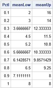
Because there are 10 observations and the program uses deciles to define the tails, each row gives the mean of the smallest and largest k observations for k=1, 2, ..., 10. For example, the second row indicates that the mean of the two smallest values is 3, and the mean of the two largest values is 14.

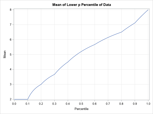
If you plot the estimated means as a function of the percentile, you can see how the functions interpolate between the data values. The following statements compute and graph the mean of the lower p_th quantile as a function of p. The graph of the mean of the upper tail is computed in an analogous fashion:

/* plot the mean of the lower tail as a function of p */
p = do(0, 1, 0.01);
mLow = j(1, ncol(p), .);
do i = 1 to ncol(p);
   mLow[i] = meanLowerPctl(p[i], x);
end;
 
title "Mean of Lower p Percentile of Data";
call series(p, mLow) grid={x y} xvalues=do(0,1,0.1) label={"Percentile" "Mean"};

Compute Hogg's skewness in SAS

With these functions, you can compute Hogg's estimate of skewness. The following SAS/IML function implements the formula. The function is then tested on a large random sample from the exponential distribution.

/* estimate of Hogg skewness */
start HoggSkew(_x);
   x = _x;
   call sort(x);
   L05 = meanLowerPctl(0.05, x);
   U05 = meanUpperPctl(0.05, x);
   m25 = mean(x, 'trim', 0.25);
   Skew_Hogg = (U05 - m25) / (m25 - L05); /* Right Skewness: Hogg (1974, p. 918) */
   return Skew_Hogg;
finish;
 
/* generate random sample from the exponential distribution */
call randseed(12345, 1);
N = 1E5;
x = randfun(N, "Expon");
Skew_Hogg = HoggSkew(x);  /* find the Hogg skewness for exponential data */
print Skew_Hogg;

The sample estimate of Hogg's skewness for these data is 4.558. The value of Hogg's skewness for the exponential distribution is 4.569, so there is close agreement between the parameter and its estimate from the sample.

Compute Hogg's kurtosis in SAS

In the same paper, Hogg (1974) proposed a robust measure of kurtosis, which is
Kurt_H = (U(0.2) – L(0.2)) / (U(0.5 - U(0.5))
where U(0.2) and L(0.2) are the means of the upper and lower 20% of the data (respectively) and U(0.5) and L(0.5) are the means of the upper and lower 50% of the data (respectively). You can use the same SAS/IML functions to compute Hogg's kurtosis for the data:

/* estimate of Hogg kurtosis */
start HoggKurt(_x);
   x = _x;
   call sort(x);
   L20 = meanLowerPctl(0.20, x);
   U20 = meanUpperPctl(0.20, x);
   L50 = meanLowerPctl(0.50, x);
   U50 = meanUpperPctl(0.50, x);
   Kurt_Hogg = (U20 - L20) / (U50 - L50); /* Kurtosis: Hogg (1974, p. 913) */
   return Kurt_Hogg;
finish;
 
Kurt_Hogg = HoggKurt(x);  /* find the Hogg kurtosis for exponential data */
print Kurt_Hogg;

For comparison, the exact value of the Hogg kurtosis for the exponential distribution is 1.805.

Summary

This article shows how to compute Hogg's robust measures of skewness and kurtosis. The article was inspired by Bono et al. (2020), who explore the bias and accuracy of Hogg's measures of skewness and kurtosis as compared to the usual moment-based skewness and kurtosis. They conclude that Hogg’s estimators are less biased and more accurate. Bono et al. provide a SAS macro that computes Hogg's estimators. In this article, I rewrote the computations as SAS/IML functions to make them more efficient and more understandable. These functions enable researchers to compute Hogg's skewness and kurtosis for data analysis and in simulation studies.

You can download the complete SAS program that defines the Hogg measures of skewness and kurtosis. The program includes computations that show how to compute these values for a distribution.

References

• Bono, R., Arnau, J., Alarcón, R., & Blanca, M. J. (2020). "Bias, precision, and accuracy of skewness and kurtosis estimators for frequently used continuous distributions," Symmetry, 12(1), 19.
• Hogg, R. (1974). "Adaptive Robust Procedures: A Partial Review and Some Suggestions for Future Applications and Theory," JASA, 69(348), 909-923.