The skewness of a distribution indicates whether a distribution is symmetric or not. The Wikipedia article about skewness discusses two common definitions for the sample skewness, including the definition used by SAS. In the middle of the article, you will discover the following sentence: In general, the [estimators]are both biased estimators of the population skewness. The article goes on to say that the estimators are not biased for symmetric distributions. Similar statements are true for the sample kurtosis.

This statement might initially surprise you. After all, the statistics that we use to estimate the mean and variance are unbiased. Although biased estimates are not inherently "bad," it is useful to get an intuitive feel for how biased an estimator might be.

Let's demonstrate the bias in the skewness statistic by running a Monte Carlo simulation. Choose an unsymmetric univariate distribution for which the population skewness is known. For example, the exponential distribution has skewness equal to 2. Then do the following:

1. Choose a sample size N. Generate B random samples from the chosen distribution.
2. Compute the sample skewness for each sample.
3. Compute the average of the skewness values, which is the Monte Carlo estimate of the sample skewness. The difference between the Monte Carlo estimate and the parameter value is an estimate of the bias of the statistic.

In this article, I will generate B=10,000 random samples of size N=100 from the exponential distribution. The simulation shows that the expected value of the skewness is NOT close to the population parameter. Hence, the skewness statistic is biased.

A Monte Carlo simulation of skewness

The following DATA step simulates B random samples of size N from the exponential distribution. The call to PROC MEANS computes the sample skewness for each sample. The call to PROC SGPLOT displays the approximate sampling distribution of the skewness. The graph overlays a vertical reference line at 2, which is the skewness parameter for the exponential distribution, and also overlays a reference line at the Monte Carlo estimate of the expected value.

%let NumSamples = 10000;
%let N = 100;
/* 1. Simulate B random samples from exponential distribution */
data Exp;
call streaminit(1);
do SampleID = 1 to &NumSamples;
   do i = 1 to &N;
      x = rand("Expo");
      output;
   end;
end;
run;
 
/* 2. Estimate skewness (and other stats) for each sample */
proc means data=Exp noprint;
   by SampleID;
   var x;
   output out=MCEst mean=Mean var=Variance skew=Skewness kurt=Kurtosis;
run;
 
/* 3. Graph the sampling distribution and overlay parameter value */
title "Monte Carlo Distribution of Sample Skewness";
title2 "N = &N; B = &NumSamples";
proc sgplot data=MCEst;
   histogram Skewness;
   refline 2 / axis=x lineattrs=(thickness=3 color=DarkRed) 
             labelattrs=(color=DarkRed) label="Parameter";
   refline 1.818 / axis=x lineattrs=(thickness=3 color=DarkBlue) label="Monte Carlo Estimate"
             labelattrs=(color=DarkBlue) labelloc=inside ;
run;
 
/* 4. Display the Monte Carlo estimate of the statistics */ 
proc means data=MCEst ndec=3 mean stddev;
   var Mean Variance Skewness Kurtosis;
run;

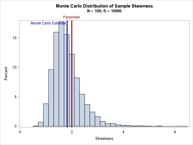
For the exponential distribution, the skewness parameter has the value 2. However, according to the Monte Carlo simulation, the expected value of the sample skewness is about 1.82 for these samples of size 100. Thus, the bias is approximately 0.18, which is about 9% of the true value.

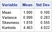
The kurtosis statistic is also biased. The output from PROC MEANS includes the Monte Carlo estimates for the expected value of the sample mean, variance, skewness, and (excess) kurtosis. For the exponential distribution, the parameter values are 1, 1, 2, and 6, respectively. The Monte Carlo estimates for the sample mean and variance are close to the parameter values because these are unbiased estimators. However, the estimates for the skewness and kurtosis are biased towards zero.

Summary

This article uses Monte Carlo simulation to demonstrate bias in the commonly used definitions of skewness and kurtosis. For skewed distributions, the expected value of the sample skewness is biased towards zero. The bias is greater for highly skewed distributions. The skewness statistic for a symmetric distribution is unbiased.