In the previous section of this series we discussed ways of assessing the relationship between variables. This week we change the focus to the shape and sparsity of our dataset.

One area of Explanatory Data Analysis  which we’ve missed so far is the impact of missingness in data. Having missing observations in a dataset can have quite significant implications for building predictive models.

The main, and perhaps most obvious, reason that missingness in your data can cause an issue is simply that there are fewer cases with which to build a reliable model which will generalise well to new data. Any missing input equates to lost information; however this can be more of a problem depending on the type of model you choose to use.

This is because many types of predictive models rely on ‘complete case analysis’. In other words, in order to train a predictive model, the model will only be able to consider a row without any missing items, so if you have a row with ten inputs and only one missing record then you lose all of the useful information from the remaining nine inputs. This applies to techniques which leverage linear methods to train models such as linear and logistic regression, support vector machines and even neural networks.

In the next section of this series we’ll consider the different types of missingness and some methods to help address missing data. In this section we’re going to focus on how missingness and dimensionality (i.e. number of model inputs) in datasets makes it harder to build a reliable model without substantially increasing the number of observations in your dataset.

The curse of dimensionality

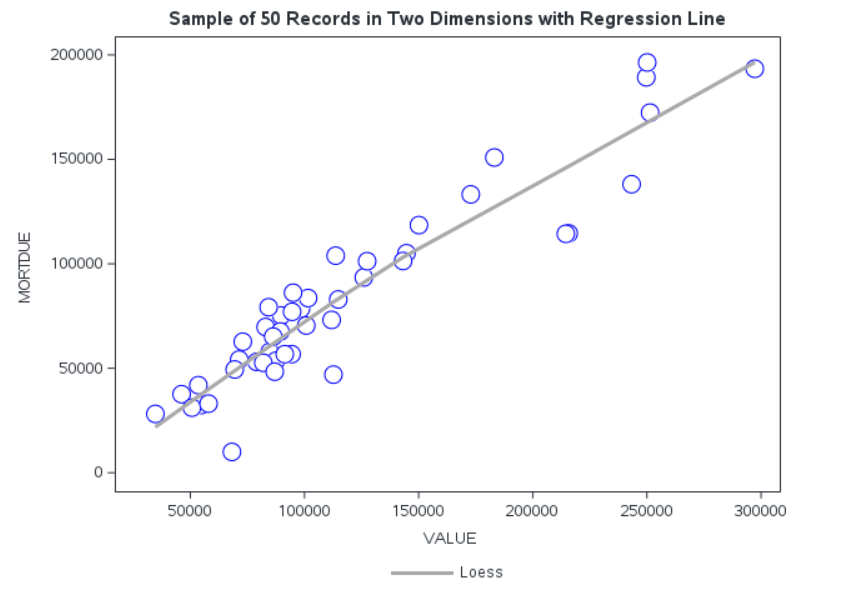
The phenomenon known as ‘The Curse of Dimensionality’ refers to the relationship between the number of observations needed to fit a model in relation to the number of inputs, or dimensions, the model uses. For example, looking at Figure 1, consider a simple linear regression with one input only has two dimensions, the input space for the model to train on is already relatively dense and a few missing values may not be an issue if you have a moderately sized dataset.

A simple regression like this is well visualized in a simple scatter plot, and because it is only a 2-D relationship the regression model can be fit with a straight, or smoothed, line. From our HMEQ dataset we saw that there was a linear relationship between VALUE and MORTDUE. If we take a small sample of the data and put this into a simple 2-D Scatter plot, then we can see that the input space is relatively dense. Just looking at the plot it looks like there is a reasonable number of observations to fit a simple regression line. There is a strong positive correlation between the two variables and if we fit a smooth regression line we can see that, on average, we expect a loan applicant’s outstanding mortgage amount to increase as the value of their property increases, which seems reasonably intuitive.

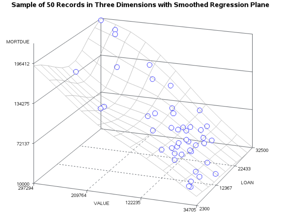
When you increase the dimensionality and extend this to two model inputs you can imagine the input space being a 3-D scatter plot, and intuitively the input space grows (a 3-D box has a larger area than a square) despite there being the same total number of observations to fill the input space.

Going back to our HMEQ dataset, using the same number of sample observations, Figure 2 shows that if we introduce another input to our scatter plot you can see that there is a lot more empty space in the plot. In other words, the input space has grown, and the observations fill the space less densely.

Once again, we are able to fit and plot a smoothed regression to describe our relationship. We see that once again we model the relationship of MORTDUE with VALUE, but this time we include the LOAN amount.

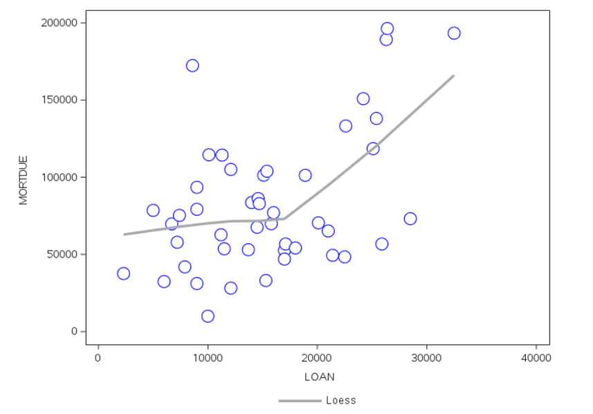
Whilst the visualization looks pretty good, it is actually quite difficult to interpret the relationship between LOAN and MORTDUE, for simplicity we can also see this isolated on a 2-D plot in Figure 3. There appears to be a fairly weak relationship between the variables which could be fit by a Spline. There appears to be only a reasonable linear relationship for loan applications greater than $20,000. Perhaps this makes sense as you would need a lot of equity to secure a larger loan amount.

Looking back at the 3-D plot you will see that we can no longer fit a line of best fit, the relationship is more complex and the regression model is fit as a plane instead. This shows us that not only do our observations less densely fill the input space, but the model complexity increases as we increase the dimensionality.

If we increase the number of inputs again it becomes something you cannot visualise and the model fit moves from being a plane to a hyper-plane. Intuitively, as the input space increases the density of the observations decrease, meaning we need more observations to fit our model.

How does this relate to missingness?

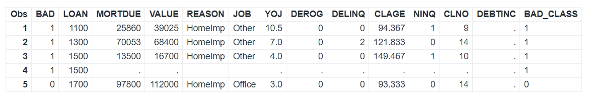
The issue of missing data further compounds the curse of dimensionality and is itself affected by the number of inputs. In real world data missingness is likely to affect only a few cells of a given observation row in your dataset. We saw in the first blog, revisited in Figure 4, that missingness varies quite a bit in our dataset, and some rows are more affected by others.

If we say, arbitrarily, that 4% of data has missing observations we can illustrate how missingness has an exponentially decaying relationship based on the number of model inputs.

Take for example our sample dataset with only 50 observations, our simple linear regression with one input will theoretically have only 2 missing values. When this expands to a model with two inputs we can consider that (0.96)² % of data are missing since the probability of input 1 and input 2 having missing values are independent of each other. By just adding one more input we now have an expected 92.16% missing cases, since our model can only use complete case analysis. When we move to three model inputs that drops again to an expected 88.47% of complete cases, meaning that of our 50 observations we expect that only 44 will be available to train our model.

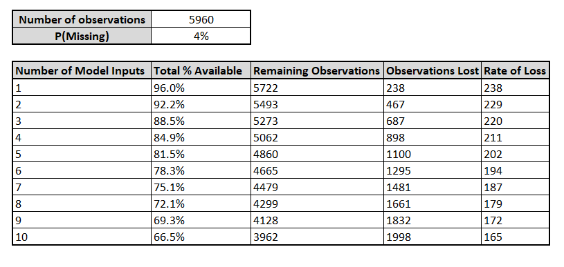
On the face of it losing only 6 observations of our 50 does not sounds so terrible. However, when we look at this from the context of our original dataset we see a much scarier picture on the potential impact of missingness. There are 10 numeric inputs available to our model, and 5,960 observations in total. If we continue to assume there is an independent 4% chance of data being missing you can see in Figure 5 that once we add all inputs we can expect to lose up to 1,998 observations from a model which relies on complete case analysis, which equates to a massive loss of 44% of our original dataset!

So, in summary, missingness can become increasingly deadly as the input space increases with the number of model inputs you use. The curse of dimensionality means that as our input space grows, we need more observations to train a model, but missingness in our data also means that as our input space grows the number of observations available to us decreases. Whilst we have focused on a regression context here, because it is easier for illustration purposes, these concepts are equally relevant to classification methods which also rely on complete case analysis.

There are some strategies to help counter this. Firstly, and rather obviously, you can simply try to use fewer inputs in your model. Though with real world data this may not be practical, since you may be dealing with data that has complex relationships in order to build a reliable model. Real world data is also not likely to have the same amount of missingness in each feature, so identifying the most affected inputs is an important task.

Secondly, you might consider opting for models which don’t require complete case analysis. Tree based techniques, for example, can handle missingness in data.

A third technique you might consider is imputation, where missing values are substituted with a replacement value. This can be a good way to leverage the useful information contained in the non-missing parts of an observation and helpful for visualization or general data analysis - though these techniques can be dangerous when used incorrectly and I generally try to avoid using imputation in a predictive model as you risk incorporating assumptions and biases into your model. This is particularly important when considering whether there is a valid reason that data is missing, we discuss this in the next section of the series.

Please also check out the SAS Users YouTube channel where fellow data scientists posted many interesting short videos on the topic.