This is the 11th installment of the "Getting Started" series. You can use penalized B-splines display a smooth curve through a set of data. The PBSPLINE statement fits spline models, displays the fit function(s), and optionally displays the data values. You can fit a wide variety of curves. You can fit a single function, or when you have a group or classification variable, fit multiple functions. (PROC SGPLOT provides a GROUP= option, whereas statistical procedures usually provide a CLASS statement that you can use to specify groups.)

The penalized B-spline software automatically picks the amount of smoothing. I like this technique a lot! It is easy to use, and it usually does a great job. We use it several places in SAS/STAT software including when displaying trace plots in Bayesian analyses. It is faster for large data sets than loess, which will be my next "Getting Started" topic. It almost always selects a reasonable amount of smoothing, and there are options you can specify if you want to change that amount. The technique was developed by Eilers and Marx (1996). I put it in PROC TRANSREG a few years later, and PROC SGPLOT calls the same code from the PBSPLINE statement.

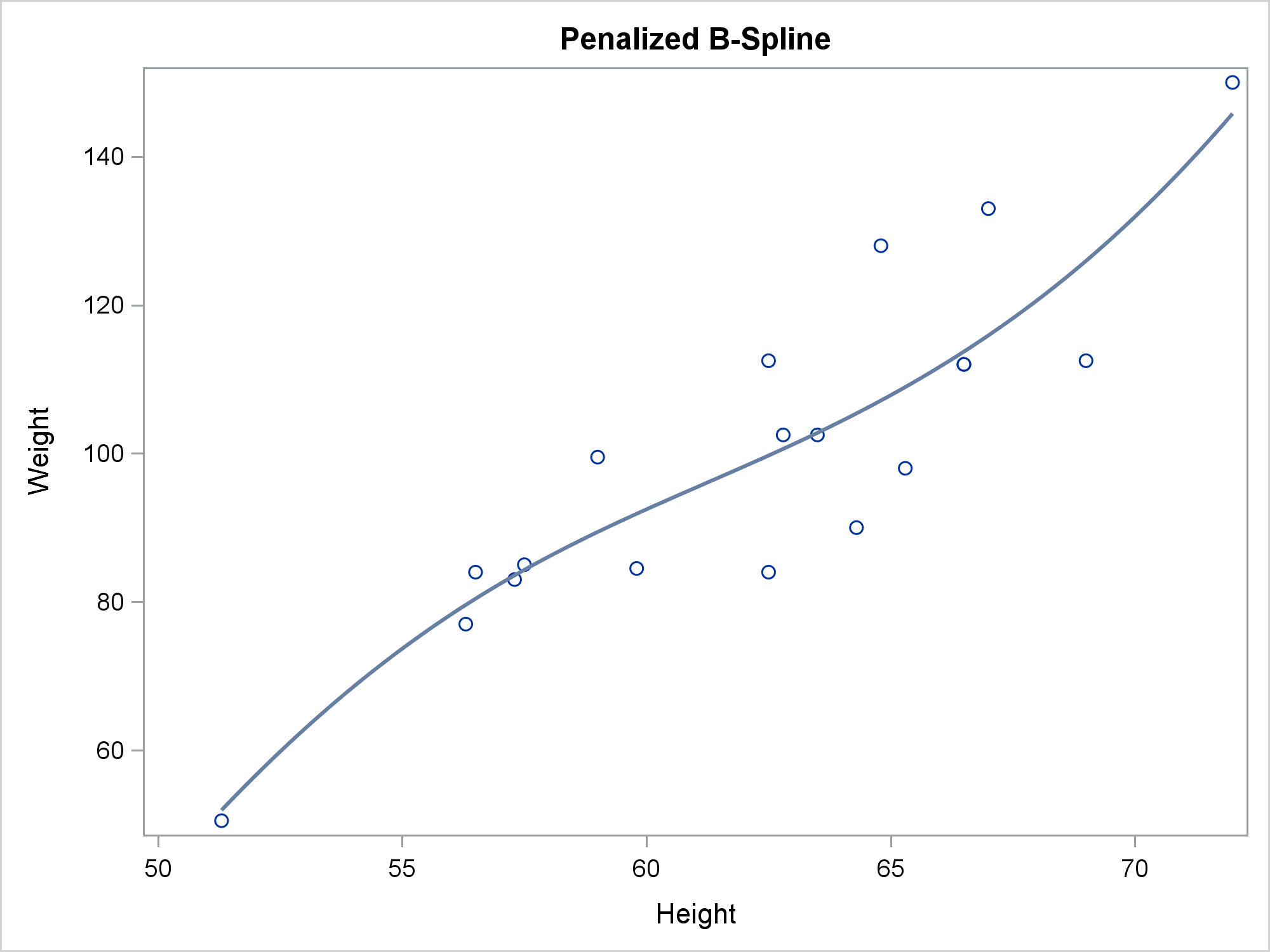
The following step displays a single curve and a scatter plot of points.

proc sgplot data=sashelp.class noautolegend;
   title 'Penalized B-Spline';
   pbspline y=weight x=height;
run;

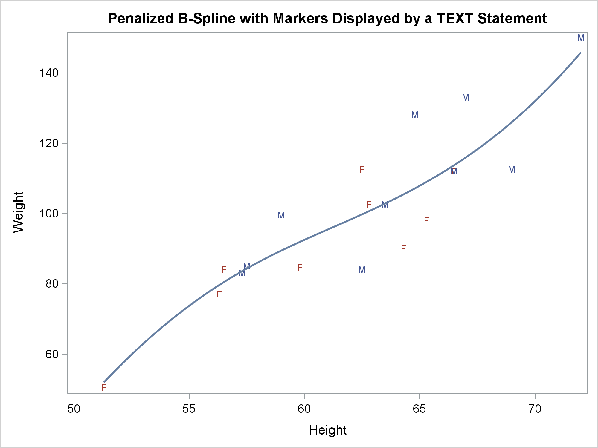
You can suppress markers by specifying the NOMARKERS option in the PBSPLINE statement. Then you can use the TEXT statement to display nondefault markers. This example uses the GROUP= and MARKERCHAR= options in the TEXT statement to differentiate the males and females.

proc sgplot data=sashelp.class noautolegend;
   title 'Penalized B-Spline with Markers Displayed by a TEXT Statement';
   text y=weight x=height text=sex / group=sex;
   pbspline y=weight x=height / nomarkers;
run;

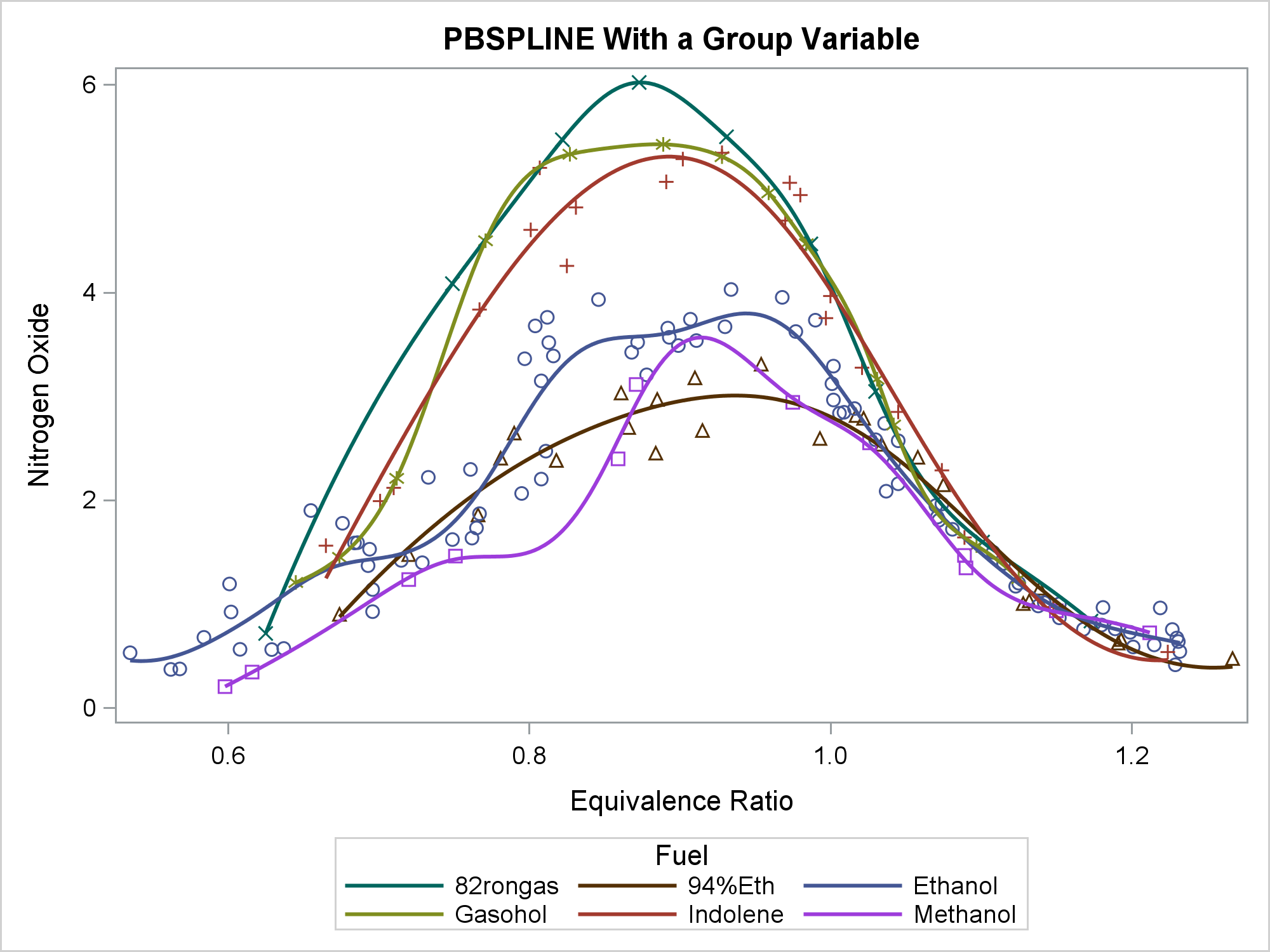
You can specify the GROUP= option in the PBSPLINE statement to get a separate fit function for each group. You can also specify ATTRPRIORITY=NONE in the ODS GRAPHICS statement and a STYLEATTRS statement to vary the markers for each group while using solid lines.

ods graphics on / attrpriority=none;
proc sgplot data=sashelp.gas;
   title 'PBSPLINE With a Group Variable';
   styleattrs datalinepatterns=(solid);
   pbspline y=nox x=eqratio / group=fuel;
run;

You can use these same techniques for groups in PBSPLINE that you can use in the REG statement.

PBSPLINE provides options that give you control over the algorithm. In most cases, you will never need to specify any of them. Options include NKNOTS=, SMOOTH=, DEGREE=, and MAXPOINTS=. By default, there are 100 evenly spaced knots and a degree 3 (cubic) polynomial. You can use SMOOTH= to specify the smoothing parameter; you might want to fit the same model by using PROC TRANSREG if you want guidance on the smoothing parameter. Again, you will mostly want to let the algorithm pick the smoothing parameter. You can specify MAXPOINTS= to control the number of points at which the spline is evaluated. I have found only two cases where might I want to change these defaults. I use PBSPLINE to chart some of my personal health history data. I find that with a small, sparse data set that consists of a few points over time, DEGREE=2 (quadratic spline) tends to work better than DEGREE=3. If you want to disable smoothing and control the smoothness by specifying the number of knots, then you can specify SMOOTH=0 and NKNOTS=k (for some nonnegative k). This last capability is why PROC SGPLOT does not provide a separate polynomial spline statement.

To see why you might want to specify DEGREE=2, NKNOTS=k for some small k, or SMOOTH=0, consider using the default options and fitting a penalized B-spline to the Sashelp.Class data set separately for each gender.

proc sgplot data=sashelp.class noautolegend;
   title 'Cubic Penalized B-Spline Is Not at Its Best With Sparse Data';
   styleattrs datalinepatterns=(solid);
   pbspline y=weight x=height / group=sex;
run;

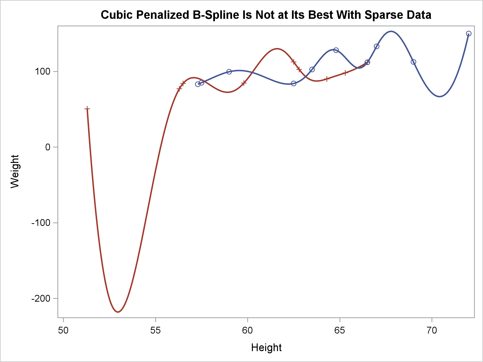
The penalized B-spline model (before smoothing) for data such as these has many more parameters than data points. The data are too sparse to support the penalized B-spline calculations, and so the results are unstable. One curve extends well outside the range of the data. Other spline techniques are subject to this same issue. You will get better results if you specify DEGREE=2 (if you want a smooth function that approximately connects the dots), NKNOTS=k for a small k such as 2-4 (if you want to fit a smooth curve through the scatter plot), or some other combination of options that ensures less overfitting.

The PBSPLINE statement contains many other options that control the appearance of the plot that you might want to change. Statistical procedures give you more control over the statistical models. PROC SGPLOT gives you an easier way to control the graph. For more options, see the documentation for the PBSPLINE statement or PROC TRANSREG.