I was searching Graphically Speaking, and I realized that we have not devoted much time to DRAW statements in the GTL. Most of our posts are devoted to PROC SGPLOT. DRAW statements provide to GTL what SG annotation provides to the SG procedures--a way to add text, shapes, images, lines, and arrows to graphs.
This post will not say much about the mechanics of DRAW statements; I will leave that for a future post. For now, I just want you to be aware that DRAW statements exist and that you can use them to add elements to graphs that analytical procedures produce. Also, you can programatically add elements to templates for a single graph or for multiple graphs. First, have you ever wondered how SG annotation works? In my previous post, I showed how to look at the graph template that PROC SGPLOT writes to better understand what PROC SGPLOT does. Let's do that again. This is a teaching example. Sometimes, one of the harder things with SG annotation is knowing what your range of coordinates are. The following steps create an SG annotation data set and use it to show the wall drawing space in PROC SGPLOT.
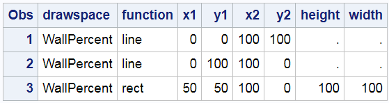
data anno;
   retain drawspace 'WallPercent';
   function = 'line     '; x1=0;  y1=  0; x2=100; y2=100;        output;
                                  y1=100;         y2=  0;        output;
   function = 'rectangle'; x1=50; y1= 50; height=100; width=100; output;
run;

proc sgplot data=sashelp.class sganno=anno tmplout='t1';
   scatter y=weight x=height;
run; |
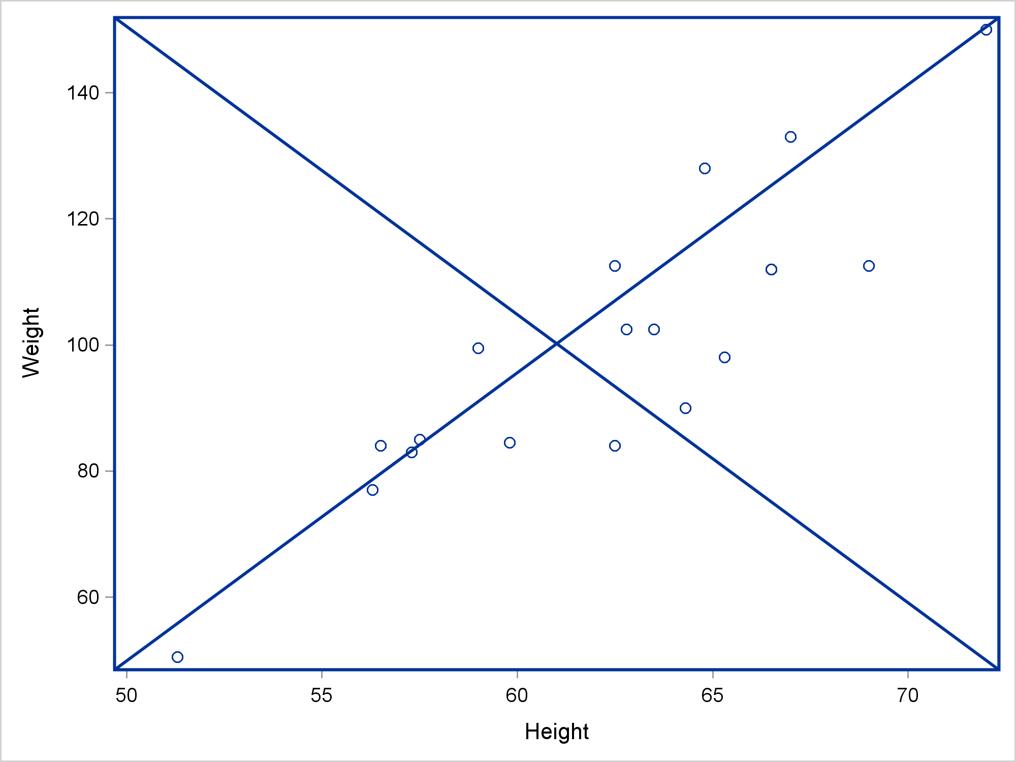
This graph clearly shows that the wall space corresponds to the space that is surrounded by the axes. WALLPERCENT coordinates range from 0 to 100, although extrapolation is always possible. The file t1 contains the graph template.
proc template;
define statgraph sgplot;
begingraph / collation=binary;
layout overlay / yaxisopts=(labelFitPolicy=Split) y2axisopts=(labelFitPolicy=Split);
   ScatterPlot X=Height Y=Weight / subpixel=off primary=true LegendLabel="Weight" NAME="SCATTER";
    DrawLine X1=0 Y1=0 X2=100 Y2=100 / DRAWSPACE=WallPercent;
    DrawLine X1=0 Y1=100 X2=100 Y2=0 / DRAWSPACE=WallPercent;
    DrawRectangle X=50 Y=50 WIDTH=100 HEIGHT=100 / DRAWSPACE=WallPercent;
endlayout;
endgraph;
end;
run; |
SG annotation works by adding DRAW statements to the template. Two DRAWLINE statements draw the line and the DRAWRECTANGLE statement draws the rectangle.
I deliberately made a mistake in the next SG annotation data set.
data anno;
   retain drawspace 'WallPercent';
   function = 'line'; x1=0; y1=  0; x2=100; y2=100; output;
                            y1=100;         y2=  0; output;
   function = 'rectangle'; x1=50; y1=50; height=100; width=100; output;
run;

proc sgplot data=sashelp.class sganno=anno tmplout='t2';
   scatter y=weight x=height;
run; |
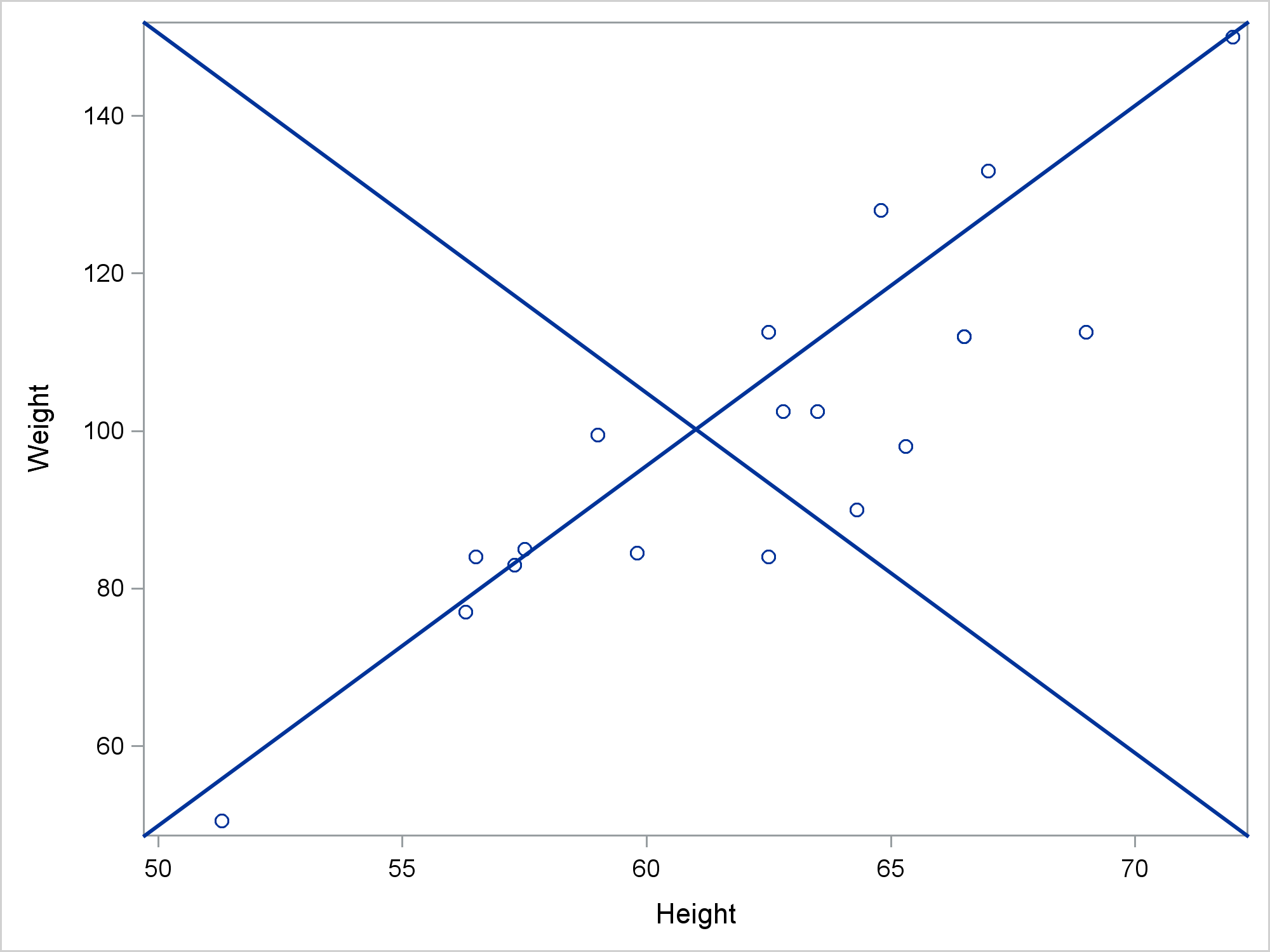
What happened to the rectangle? Here is the template.
proc template;
define statgraph sgplot;
begingraph / collation=binary;
layout overlay / yaxisopts=(labelFitPolicy=Split) y2axisopts=(labelFitPolicy=Split);
   ScatterPlot X=Height Y=Weight / subpixel=off primary=true LegendLabel="Weight" NAME="SCATTER";
    DrawLine X1=0 Y1=0 X2=100 Y2=100 / DRAWSPACE=WallPercent;
    DrawLine X1=0 Y1=100 X2=100 Y2=0 / DRAWSPACE=WallPercent;
endlayout;
endgraph;
end;
run; |
There is no DRAWRECTANGLE statement. Let's look at the SG annotation data set.
proc print; run; |
The 'Rectangle' value of the Function variable was truncated. You either need to pad the first value by using blanks or use a LENGTH statement. While it is easiest to simply look at the SG annotation data set, the template does provide some clues about what is happening. It is perfectly normal for SG annotation to ignore anything that it does not understand.
Now that we see that SG annotation writes DRAW statements, let's look at how you can add SG annotation statements to graphs that analytical procedures produce. The next few examples will be like the first example--they illustrate drawing spaces more than anything else. We will use PROC KDE because it has one of the simplest templates in SAS, which makes a simple scatter plot. While you can always display the template, copy it, and manually edit it, I prefer to show you how to programatically modify the template. You begin by deleting any compiled template that might be left over from previous work. The DELETE statement generates a warning if there is no template to delete, but that is not a problem. The SOURCE statement writes the template to a file, temp1.tmp.
proc template; delete Stat.KDE.Graphics.ScatterPlot / store=sasuser.templat; source Stat.KDE.Graphics.ScatterPlot / file='temp1.tmp'; quit; |
The following step creates a data set that contains four DRAW statements.
data draw; length line $ 256; input; line = _infile_; datalines4; drawline x1=0 y1= 0 x2=100 y2=100; drawline x1=0 y1=100 x2=100 y2= 0; drawrectangle x=50 y=50 height=100 width=100; drawtext 'Center' / x=50 y=50; ;;;; |
This step processes the template in temp1.tmp.
data _null_;
   infile 'temp1.tmp';
   input;
   if _n_ = 1 then
      call execute('proc template;');
   call execute(_infile_);
   if find(lowcase(_infile_), 'layout overlay') then lo + 1;
   if lo and index(_infile_, ';') then do;
      lo = 0;
      do i = 1 to ndraws;
         set draw point=i nobs=ndraws;
         call execute(line);
      end;
   end;
run; |
It finds the LAYOUT OVERLAY statement. Then it finds the semicolon that ends the LAYOUT OVERLAY statement. (The statement might be continued onto two or more lines.) When the DATA _NULL_ step finds a LAYOUT OVERLAY statement, it adds all of the DRAW statements. It sets the LAYOUT OVERLAY flag variable to 0 and continues processing the other lines in the template. Finally, PROC KDE creates a graph that uses the modified template.
proc kde data=sashelp.class; ods select scatterplot; bivar height weight / plots=scatter; run; |
The graph shows that the default drawing space is LAYOUTPERCENT, which extends from the edge of the axis label to the opposite axis.
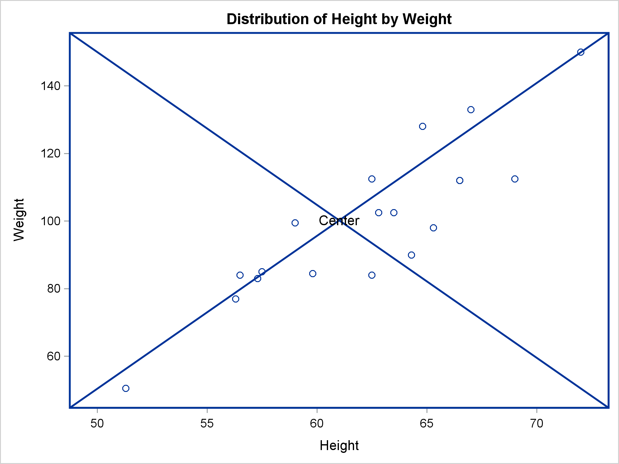
The following step uses an assignment statement to add a common option to all statements. It sets the drawing space to GRAPHPERCENT.
data draw;
   length line $ 256;
   input;
   line = catx(' ', _infile_, ifc(find(_infile_, '/'), ' ', '/'), 'drawspace=GraphPercent;');
   datalines4;
drawline x1=0 y1=  0 x2=100 y2=100
drawline x1=0 y1=100 x2=100 y2=  0
drawrectangle x=50 y=50 height=100 width=100
drawtext 'Center' / x=50 y=50
;;;; |
The next step finds a BEGINGRAPH statement rather than a LAYOUT OVERLAY statement, and inserts the DRAW statements after it. PROC KDE makes the graph.
data _null_;
   infile 'temp1.tmp';
   input;
   if _n_ = 1 then
      call execute('proc template;');
   call execute(_infile_);
   if find(lowcase(_infile_), 'begingraph') then bg + 1;
   if bg and index(_infile_, ';') then do;
      bg = 0;
      do i = 1 to ndraws;
         set draw point=i nobs=ndraws;
         call execute(line);
      end;
   end;
run;

proc kde data=sashelp.class;
   ods select scatterplot;
   bivar height weight / plots=scatter;
run; |
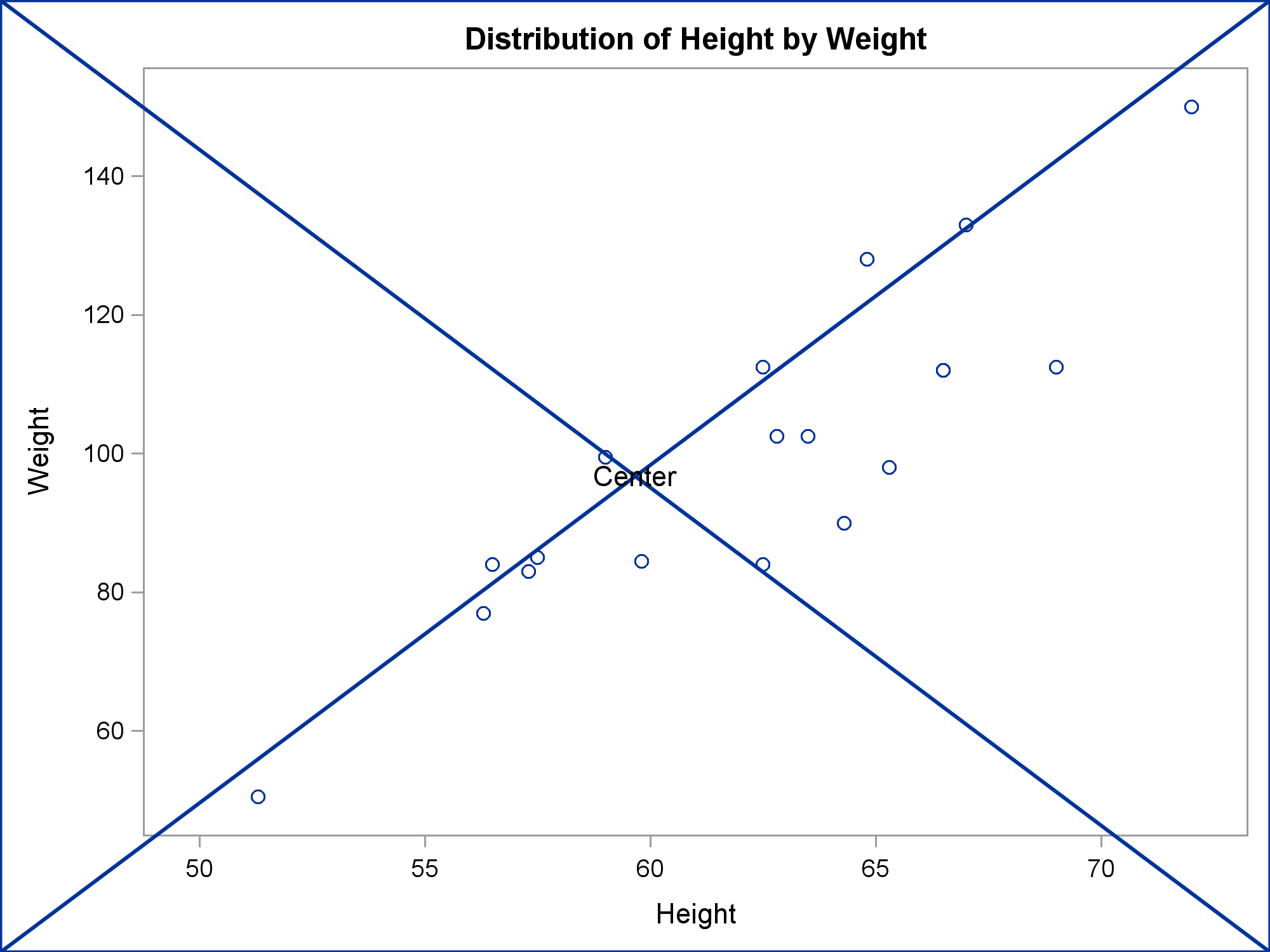
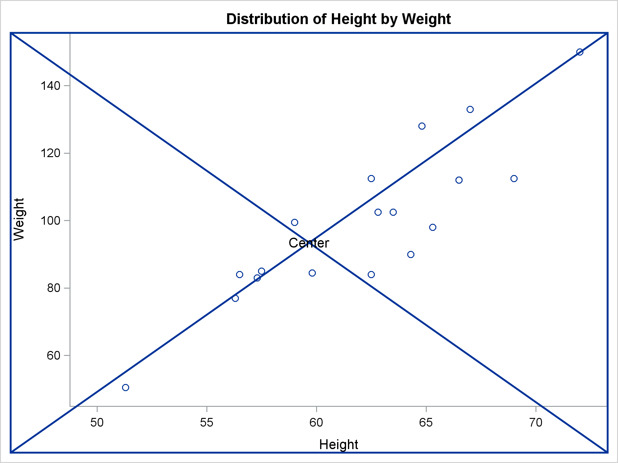
These next steps use WALLPERCENT coordinates and insert the DRAW statements after the LAYOUT OVERLAY statement.
data draw;
   length line $ 256;
   input;
   line = catx(' ', _infile_, ifc(find(_infile_, '/'), ' ', '/'),
              'drawspace=WallPercent;');
   datalines4;
drawline x1=0 y1=  0 x2=100 y2=100
drawline x1=0 y1=100 x2=100 y2=  0
drawrectangle x=50 y=50 height=100 width=100
drawtext 'Center' / x=50 y=50
;;;;

data _null_;
   infile 'temp1.tmp';
   input;
   if _n_ = 1 then
      call execute('proc template;');
   call execute(_infile_);
   if find(lowcase(_infile_), 'layout overlay') then lo + 1;
   if lo and index(_infile_, ';') then do;
      lo = 0;
      do i = 1 to ndraws;
         set draw point=i nobs=ndraws;
         call execute(line);
      end;
   end;
run;

proc kde data=sashelp.class;
   ods select scatterplot;
   bivar height weight / plots=scatter;
run; |
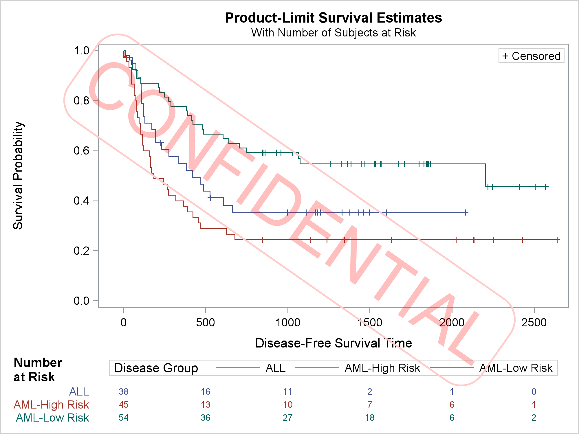
These steps show how you can add DRAW statements to the Kaplan-Meier plot. Also see the SAS/STAT chapter Customizing the Kaplan-Meier Survival Plot for other ways. (You can add DRAW statements by using the %StmtsBeginGraph macro that is discussed in this chapter.) This example adds a header over the row labels in the at-risk table and adds a "CONFIDENTIAL" water mark.
proc template;
   delete Stat.Lifetest.Graphics.ProductLimitSurvival2 / store=sasuser.templat;
   source Stat.Lifetest.Graphics.ProductLimitSurvival2 / file='temp2.tmp';
quit;

data draw;
   length line $ 256;
   input;
   line = _infile_;
   datalines4;
drawtext      textattrs=(weight=Bold) 'Number at Risk' / x=5 y=2 width=9;
drawtext      textattrs=(color=red size=52pt)
              'CONFIDENTIAL' / transparency=0.75 rotate=-35
              width=110 justify=center;
drawrectangle x=50 y=50 width=90 height=30 / cornerradius=0.5 rotate=-35
              outlineattrs=(color=cxFFCCCC);
;;;;

data _null_;
   infile 'temp2.tmp';
   input;
   if _n_ = 1 then
      call execute('proc template;');
   call execute(_infile_);
   if find(_infile_, 'layout lattice') then lo + 1;
   if lo and find(_infile_, 'layout overlay') then lo + 1;
   if lo eq 2 and index(_infile_, ';') then do;
      lo = 0;
      do i = 1 to ndraws;
         set draw point=i nobs=ndraws;
         call execute(line);
      end;
   end;
run;

proc lifetest data=sashelp.BMT plots=survival(atrisk outside maxlen=13);
   ods select survivalplot;
   time T * Status(0);
   strata Group;
run; |
The DATA _NULL_ step finds LAYOUT LATTICE statements, then finds the first LAYOUT OVERLAY statement within a LAYOUT LATTICE, then finds the end of that statement. It inserts the DRAW statements after that. It can potentially insert the DRAW statements into multiple overlays.
The next example shows how to insert multiple DRAW statements into multiple overlays.
data draw;
   length line $ 256;
   input;
   line = catx(' ', _infile_, ifc(find(_infile_, '/'), ' ', '/'),
              'drawspace=WallPercent;');
   datalines4;
drawline x1=0 y1=  0 x2=100 y2=100
drawline x1=0 y1=100 x2=100 y2=  0
drawrectangle x=50 y=50 height=100 width=100
drawtext 'Center' / x=50 y=50 width=30
;;;;

proc template;
   delete Stat.Princomp.Graphics.ScreePlot2 / store=sasuser.templat;
   source Stat.Princomp.Graphics.ScreePlot2 / file='temp3.tmp';
quit;

data _null_;
   infile 'temp3.tmp';
   input;
   if _n_ = 1 then
      call execute('proc template;');
   call execute(_infile_);
   if find(lowcase(_infile_), 'layout overlay') then lo + 1;
   if lo and index(_infile_, ';') then do;
      lo = 0;
      do i = 1 to ndraws;
         set draw point=i nobs=ndraws;
         call execute(line);
      end;
   end;
run;

proc princomp data=sashelp.iris;
   ods select screeplot;
run; |
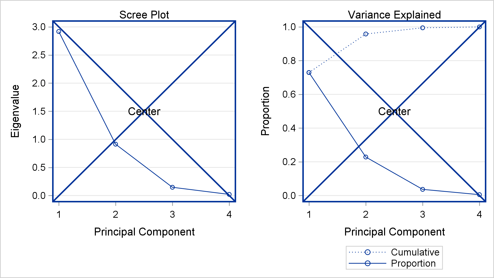
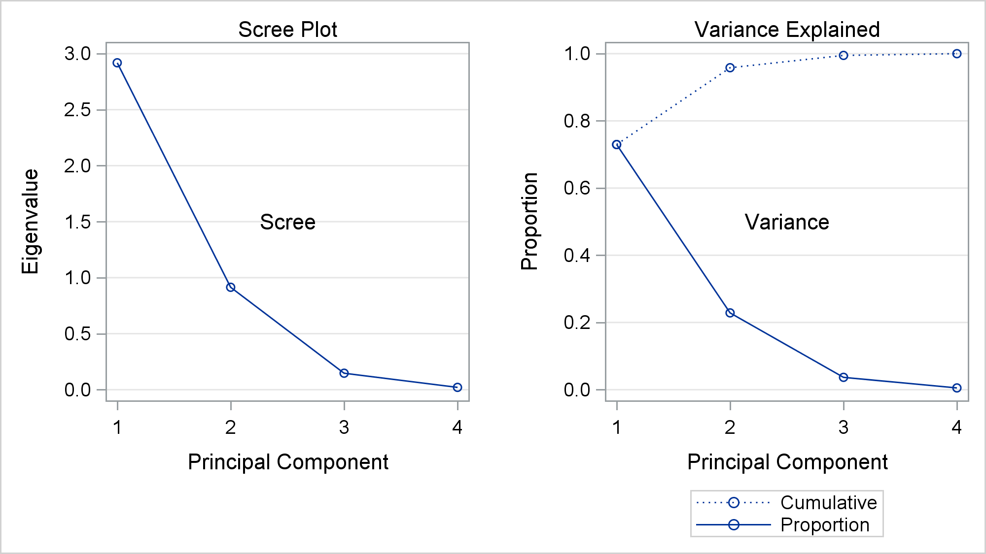
The final example assigns a group number to each statement, and inserts Group=1 statements into the first overlay and Group=2 statements into the second overlay.
data draw;
   length line $ 256;
   input;
   line = catx(' ', _infile_, ifc(find(_infile_, '/'), ' ', '/'), 'drawspace=WallPercent;');
   group = _n_;
   datalines4;
drawtext 'Scree' / x=50 y=50 width=30
drawtext 'Variance' / x=50 y=50 width=30
;;;;

data _null_;
   infile 'temp3.tmp';
   input;
   if _n_ = 1 then
      call execute('proc template;');
   call execute(_infile_);
   if find(lowcase(_infile_), 'layout overlay') then do;
      lo + 1;
      lonum + 1;
   end;
   if lo and index(_infile_, ';') then do;
      lo = 0;
      do i = 1 to ndraws;
         set draw point=i nobs=ndraws;
         if group eq lonum then call execute(line);
      end;
   end;
run;

proc princomp data=sashelp.iris;
   ods select screeplot;
run; |
While I do not show it, you can use PROC TEMPLATE and the SOURCE statement and not specify a full path. You can then programatically process multiple templates.
proc template; source Stat.Princomp / file='temp4.tmp'; * Process all PRINCOMP templates; source Stat / file='temp5.tmp'; * Process all STAT templates; quit; |
For more information about DRAW statements, see the documentation or check back for future posts.
