We continue my colleague Udo Sglavo's example with the SAS code for incorporating R models into SAS Forecast Server:
 Code for Including R Model Results in SAS
As a first step I’m exporting a data set containing one time series from SAS to R (actually I will use the same data as for the cross-validation experiment: data set A10 (“Monthly sales of anti-diabetic drugs in Australia”) – as I would like to compare the forecasting methods using the last 12 month as out-of-sample data, I’m splitting the data first before passing it to R).
data work.fitregion outofsample; set work.a10 end=last; date=intnx("month","01JUL91"d,var1-1); rename var2=actual; drop var1; format date date9.; if date gt "01JUN2007"d then output outofsample; else output fitregion; run; data export; set fitregion(drop=date); run; |
As a next step PROC IML is run to access Hyndman’s ETS model in R. Note that between the submit block R code is used. The resulting matrix of ETS is reimported to SAS. Due to my poor understanding of ETS in R I’m assuming that there is not a single object which contains both the fit and the forecasted value. As such I’m importing 2 data sets.
ods results off; proc iml; call ExportDataSetToR("work.export", "region"); submit /r; library(fpp) newdata <- ts(region, frequency = 1, start = c(1991,7)) fit <- ets(newdata) tmp1 <- forecast(fit,h=12) tmp2 <- fitted.values(fit) endsubmit; call ImportMatrixFromR(tmp1, "tmp1"); create work.predict from tmp1[colname={"Predict" "L95" "U95" "L99" "U99"}]; APPEND FROM tmp1; call ImportMatrixFromR(tmp2, "tmp2"); create work.fit from tmp2[colname={"Predict" "Date"}]; APPEND FROM tmp2; quit; |
After importing the results from R I’m creating a data set which can be used in SAS High-Performance Forecasting as an external model input. Also I’m adding back the out of sample data.
data r_fit; merge fitregion(keep=date) fit; run; data predict; retain i; set predict; i+1; date=intnx("month","01JUN2007"d,i); format date date9.; run; data r_predict; merge fitregion r_fit predict outofsample; by date; drop i; run; |
Also I’m creating a model repository, which will allow me to include the R model in the SAS High-Performance Forecasting run.
ods results; proc hpfexmspec modelrepository=work.repository specname=external_r speclabel="R ETS Model"; exm nparms=3; run; proc hpfselect modelrepository=work.repository selectname=select; specification external_r/exmmap(predict=predict lower=L95 upper=U95); run; |
Then I’m running the diagnostic engine called HPFDIAGNOSE to let it figure out the appropriate models automatically. Note that I’m leaving out 12 periods as out of sample data. Also I let HPFDIAGNOSE decide which ARIMA, UCM or ESM formulation makes the most sense for the data at hand.
proc hpfdiagnose data=r_predict modelrepository=work.repository inselectname=select outest=work.est back=12 criterion=MASE; id date interval=month; forecast actual; esm;arimax;ucm; run; |
As a last step I’m running the HPFENGINE to pick the model which performs best (using the three SAS models and the R ETS model). I’m using MASE as a selection statistic and again I’m using 12 month as out-of-sample data.
proc hpfengine data=r_predict modelrepository=work.repository task=select(criterion=MASE override) inest=work.est out=_null_ outfor=outfor back=12 lead=12 print=select plot=forecasts; id date interval=month; forecast actual; external predict; run; |
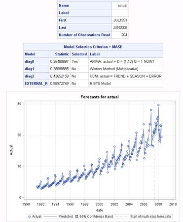
The resulting model selection table and the forecasts plots look like this:
In this particular case the ARIMA model outperforms all other models – which is in line with the findings of the cross-correlation exercise I published earlier.

