My first post on customer journey optimization set the scene by introducing the concept of marketing as a game to be won. The rules to this game are complex, some are known, and others can be learned. Above all, the game is built on a shifting landscape of customer, competitor and market dynamics. Winning this game requires a flexible and dynamic approach. I argued that emerging AI-based technologies provide a step up in sophistication of approach to finding winning strategies.

Post two provided more details on the approach SAS is taking towards using AI-based techniques such as reinforcement learning (RL) that are behind customer journey optimization. In this post, I have collaborated with my colleague Stefan Beskow from our Advanced Analytics Division to capture the essence of one method, Q-Learning, and its application to customer journeys.

Q learning

I touched on Q learning in the previous post, but now I want to show you how it can be used to optimize customer journeys. Q learning is one technique used for performing RL. There are two parts to Q learning. The first determines what action to take from a given state (current circumstances) to achieve some goal. The second part uses the response from the environment, after the action is taken, to update the state action value. By updating the value of the action, the algorithm can make a better future decision when it encounters that same state.

In journey optimization, a state action value represents the total discounted future reward received if an action is taken from a particular state. It also considers associated costs (e.g., the cost of presenting creatives) and a possible conversion at the end of the journey.

All state action values start at zero because it is difficult to predict how visitors will respond to different sequences of creatives, and in the beginning offers are made at random.

Epsilon-Greedy algorithm

To select an action to perform on a state, Q learning uses an epsilon-Greedy algorithm. This algorithm selects (with probability epsilon) a random action, and also selects with probability (1 – epsilon) the action with the highest state action value. Epsilon is a value between 0 and 1 – usually closer to 0 than 1, meaning that the chosen action is the one with the highest value at that moment

Occasionally, however, it will select a random action to determine if there are actions that may perform better. This helps to avoid dead ends and keep the system fresh. It can also help deal with changing underlying environmental conditions.

The second part of the Q-learning algorithm keeps track of the actions taken and whether they lead to a future payoff. A simplified way of looking at how it does this is to look at actions and state transitions as links in one or several chains towards eventual conversion. Some of these chains become linked and end in a conversion. When this happens, some of the conversion value gets fed back through the links in the chain(s). The amount of the conversion that get shared back is governed by a parameter called the discount factor.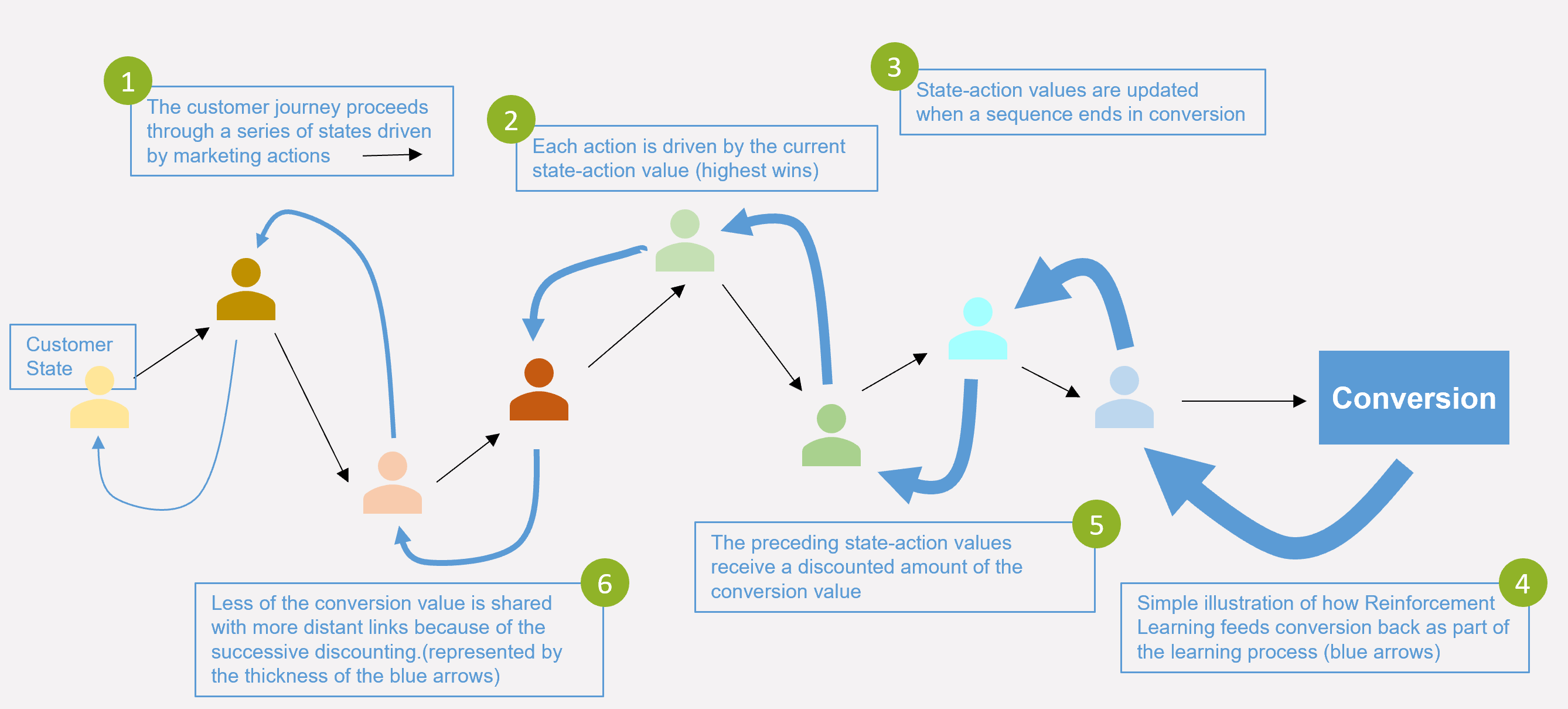

 

The above simplified diagram looks at how conversion value gets fed back to update the state-action values for a single journey path and for states that have already occurred. The thickness of the blue arrows represents the amount of conversion value that flows back. As you see, these arrows get thinner with each step backwards. This is because each step applies a discount factor to the preceding value. The discount factor is multiplicative (like a financial interest rate calculation) and has a value between (0, 1). The practical benefit of having this parameter in the model is that it allows you to tune the system to focus more on short term goals (small discount factor) or long-term goals (big discount factor).

The real picture is a lot more complex than the simple diagram above. The system must estimate the state action values for all the states that represent customers and their journeys. There are many different paths and several possible marketing actions. Some of the paths lead to conversion, and paths can be interconnected. One of the beauties of the RL approach is that the whole system is represented as a matrix, rows representing the states, columns the actions and the contents of the cells are the state action values. Each iteration is reduced to a matrix calculation to update the state-action values. Remember that the state-action values are used to make decisions as to what marketing action is taken for a given customer state.

Q learning in practice

The diagram below illustrates how the algorithm learns and applies the learning in future. Let’s suppose the system has been running for a while and that a customer arrives at the light green touchpoint. The way that the Q learning algorithm works is that most of the time they would get the action with the highest action value (action C here). Occasionally a random action is taken (with probability epsilon).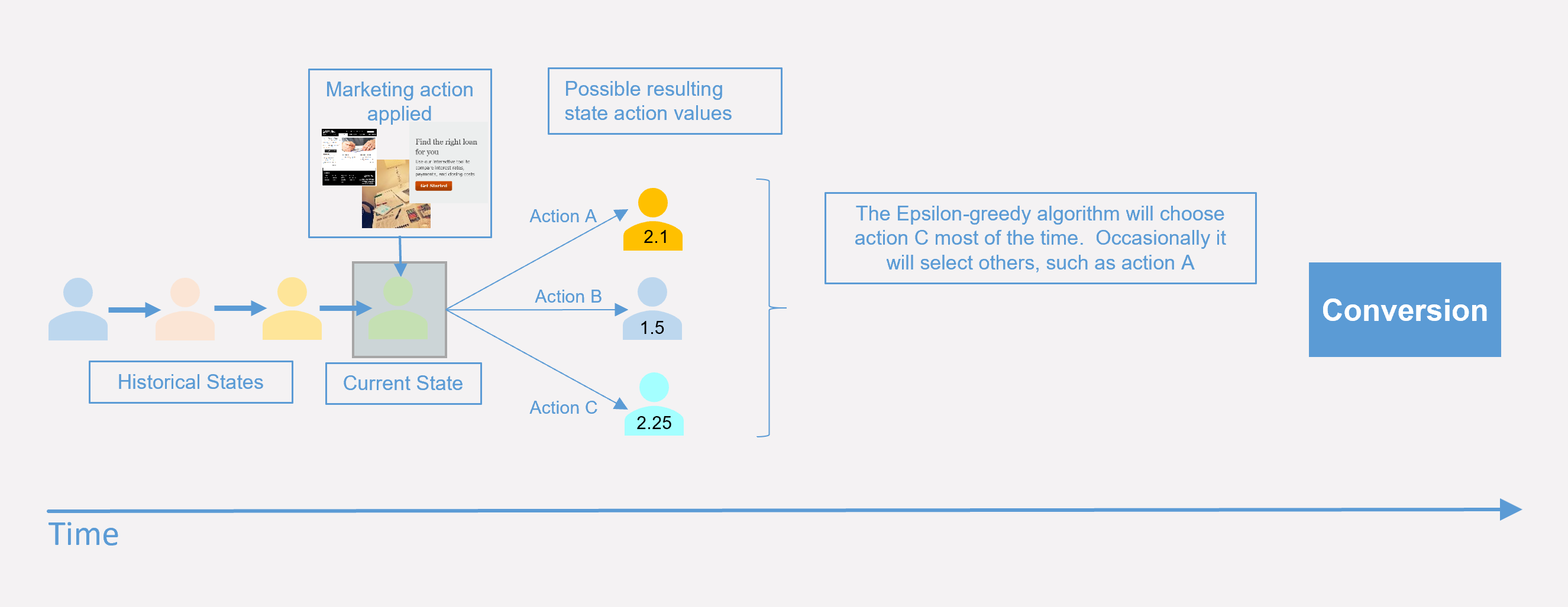

 

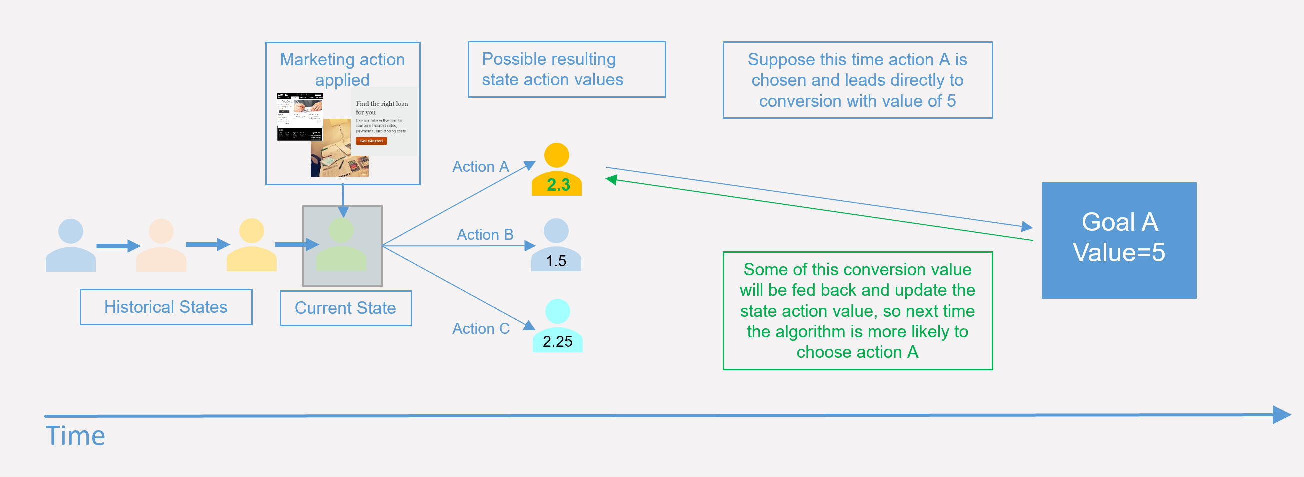
Suppose that this time action A is selected at random. For illustration, assume that it leads to a direct conversion with a value of 5.

Without going into the mathematics, the concept behind the Q-learning algorithm is that the state-action value associated with action A gets updated with a proportion of the conversion value, determined partly by the discount factor. Suppose that 0.2 out of the conversion value of 5 gets added to the orange state-action value. Next time a customer is in the same state action A will be the winner. In this way, the system has been updated by a new result.

 

Understanding why the value of the orange state action increases by 0.2 in this case is beyond the scope of this post. More details on the mathematics behind RL, and our approach to customer journey optimization will be provided in a future post. There are also excellent resources available online to aid with an understanding of how RL works.

Learn first, then exploit

You’ve seen how the epsilon parameter controls the tradeoff between continuing to learn and exploiting what has been learned. When the system serves random content, the AI is learning what happens. The AI is exploiting when it serves content based on the discovered state-action values. The most basic way to exploit the system is to reference a large lookup table containing all state-action values. But this approach rapidly becomes impractical because, just like the journey paths, the size of this state-action value table grows exponentially.

The second phase in the journey optimization approach, is developing a scalable way to score each customer state-action pair. The basis of this is to use information about observed visitor behavior to train a deep-learning model. The deep-learning model is used to estimate (score) state-action values. Having a scoring approach means that you no longer have to store and lookup a huge table, making it more computationally efficient. Another significant advantage is that it also provides a means to assign a value to a state-action pair that has not been seen before, so you can extend journey optimization to even more combinations.

RL holds great promise

The description above is a simplification of the process. But the important point is that RL is a scalable way to explore an environment that has a large number of possible combinations, far more than a human being or even conventional machine-learning techniques could analyze. The combinatorics behind potential customer journeys are a good match to the strengths of the RL algorithm, which means that this is an approach holding great promise for the future.

The initial application of RL to customer journey optimization is to determine the best sequence of creatives to show to different visitors. This is different from existing spot personalization techniques that are based on testing, or even the upcoming goal prediction task because it is the event sequence and long-term objective, rather than immediate individual message, that is being optimized.

This is the start of an exciting journey in its own right – the application of AI to marketing decision making. We are applying these techniques to well-defined business problems, such as determining the optimum sequencing of content on a web page, or of the timing of a set of emails. More macro level optimizations include which candidate activities to select for a customer at a given time, where an activity is itself a set of marketing tasks with connecting logic.

Whatever the use case, the future is bright because we have more and better tools to tackle existing as well as new marketer challenges. I hope that this three-part series of posts succeeded in providing some transparency around the techniques to show that SAS has the know-how to back up our AI story and to give you a peek behind the wizard’s curtain.