Optimize spare parts inventory under uncertainty with SAS: A simulation-based approach

Authors: Bahar Biller, Jagdishwar Mankala, and Jinxin Yi

Managing spare parts inventory is a critical aspect of asset performance management, especially in industries where equipment downtime is costly. This post, based on a real-world project with a major aircraft manufacturer, explores how to optimize spare parts inventory under uncertainty. We use a simulation-based approach with the SAS DATA step. This is a fundamental component of the SAS programming language available in all SAS products that support Base SAS functionality, including SAS Viya and SAS Viya Workbench.

Why predictive maintenance needs smart inventory planning

Predictive maintenance aims to maximize asset uptime while minimizing excess inventory of spare parts. However, there is often high uncertainty surrounding when an asset might fail. This often results in holding more inventory than necessary. Therefore, it is crucial to incorporate this uncertainty into spare parts inventory planning. This is done by accurately predicting asset lifetime distributions and leveraging the resulting uncertainty quantification to optimize spare parts management.

In Asset Performance Management with SAS, we modeled asset lifetimes by using a Weibull distribution via PROC LIFEREG and validated it with PROC LIFETEST. This post builds on that foundation by using the predicted Weibull distribution – defined by its scale and shape parameters – to optimize spare parts inventory. Our approach combines statistical modeling with stochastic simulation to account for failure-time uncertainty. By simulating various scenarios, we evaluate two key performance metrics, availability and backlog. Availability is the percentage of asset removals (failures) which can be replaced from inventory without delay. Backlog is the number of failures that cannot be addressed immediately due to insufficient stock. The analysis of these scenarios helps identify optimal inventory levels that balance cost, risk, and service level requirements in the face of uncertainty.

Use case: Fleet inventory optimization

We consider a fleet of assets where each asset is removed from operation upon failure. We track these removal events. The data set records the operating hours between them. We also assume that access to the unit cost and order lead time is available. For example, consider a unit with a cost of $1 and a lead time of 120 days. We target a 95% average availability rate. This means 95% of asset removals are expected to be immediately fulfilled from on-hand inventory. This metric is known as the Type 1 service level or fill rate, a key performance indicator (KPI) in spare parts management. We will describe how to determine the optimal inventory level that achieves this target at minimal cost. We accomplish this by utilizing the SAS DATA step for stochastic simulation and leveraging SAS analytics to support operations.

The data-driven analytics approach to inventory planning

Figure 1 illustrates a holistic approach to spare parts inventory management by integrating descriptive, predictive, and prescriptive analytics. Descriptive analytics uncover trends in historical fleet data. Predictive analytics forecasts asset failures and future inventory needs. Prescriptive analytics, which is our focus, recommends optimal inventory levels based on these forecasts. This data-driven approach strikes a balance between cost efficiency and service-level targets, enabling smarter inventory decisions.

Optimizing spare parts inventory - Figure 1: A holistic approach to spare parts inventory management — Figure 1: A holistic approach to spare parts inventory management

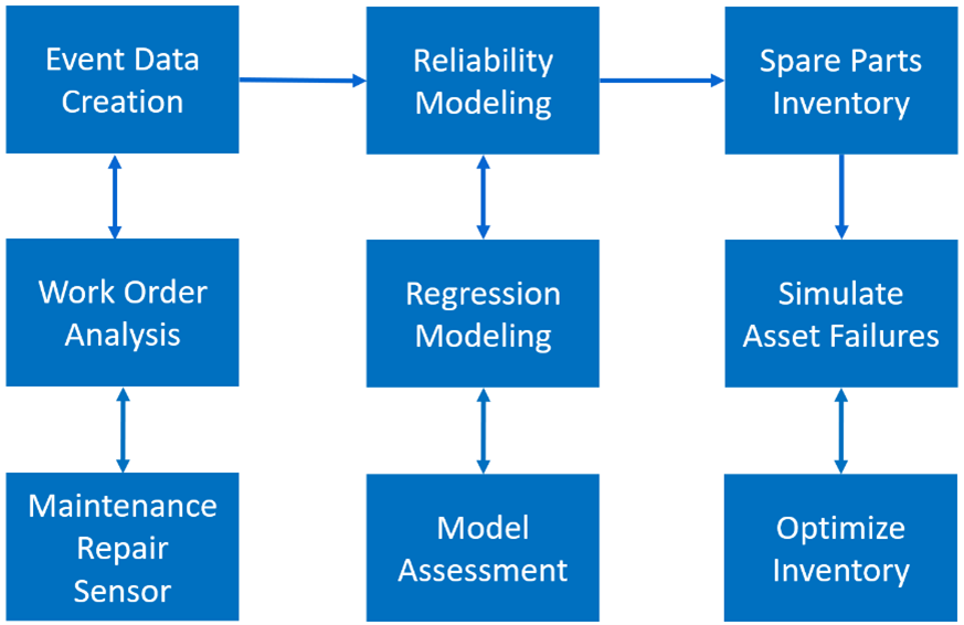
Figure 2 outlines the key steps in building a robust spare parts inventory management solution. Event data creation analyzes work orders and maintenance records to compile a history of asset failures. Reliability modeling utilizes regression techniques to estimate the distributions of asset lifetimes. We are focusing now on the final step: spare parts inventory. Here, stochastic simulation of asset failures helps determine the optimal inventory level while accounting for failure-time uncertainty.

Optimizing Spare Parts Inventory - Figure 2: Development steps for a spare parts inventory management solution — Figure 2: Development steps for a spare parts inventory management solution

How the simulation works: Inputs, logic, and outputs

Figure 3 shows the simulation-based process for optimizing spare parts inventory. It begins with collecting fleet parameters, such as annual usage hours, fleet size, and planning horizon, along with inputs like lead time, unit cost, and Weibull parameters that represent asset reliability. The simulation models random asset failures by sampling usage hours from the estimated Weibull distribution by using the rand function, specifically with the statement rand ('Weibull’, shape, scale). This generates realistic failure times by building on a uniform random number generator and utilizing the power of the SAS DATA step to simulate asset removals. For those interested in building similar simulations, Simulating Data with SAS by Rick Wicklin is an excellent resource.

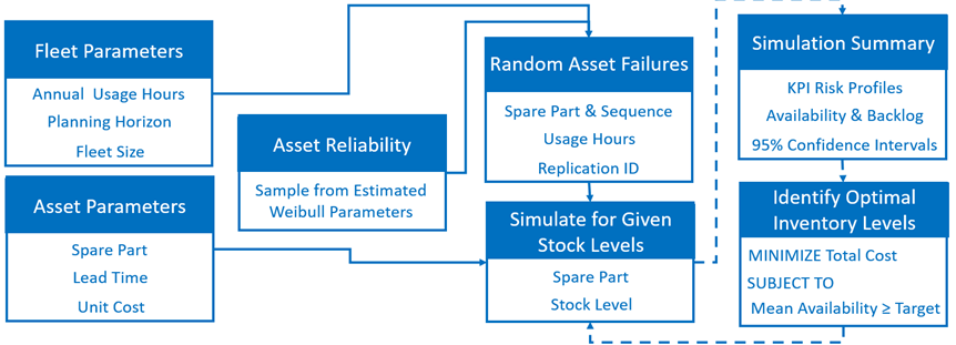
Optimizing Spare Parts Inventory - Figure 3: Simulation workflow for inventory planning — Figure 3: Simulation workflow for inventory planning

The model evaluates different inventory levels by simulating how stock changes in response to failures under a given inventory management strategy. We post-process simulation outputs to generate risk profiles for availability and backlog. This offers insight into potential future outcomes. For each metric, we calculate a 95% confidence interval that covers its unknown average value with 0.95 probability. This serves as a measurement of the error in the simulation outputs. By comparing these results across inventory levels, we identify the inventory level that minimizes cost while meeting target availability under uncertainty.

For example, we assume a fleet of five assets. Each operates 6,000 hours annually with an average utilization of 68.5% over a 365-day planning horizon. Additional input parameters include a unit cost of $1, a 120-day order lead time, and Weibull parameters: scale = 3,241.2 and shape = 1.5019. By using these inputs, the simulation performs two major tasks: (1) simulates random asset failures based on the Weibull distribution, and (2) generates inventory and backlog trajectories showing how stock levels evolve over time.

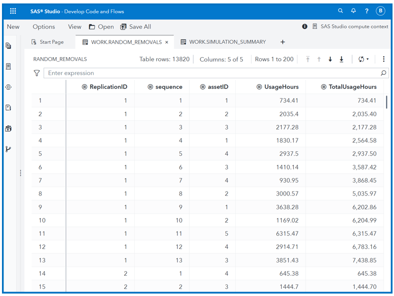
The simulation runs 1,000 replications, each representing a possible future scenario. Figure 4 shows the first 15 rows of simulated asset removals, comprising the first 13 rows from replication 1 and the last 2 rows from replication 2. The full Random_Removals data set contains 13,820 rows, with each replication generating a varying number of removals within the 365-day horizon. For instance, replication 1 has 13 removals, while replication 74 has the most at 21. This variability reflects the stochastic nature of asset failures, illustrating how uncertainty unfolds over time.

Each row in Figure 4 represents a simulated asset removal. Times between failures (UsageHours) are generated from the Weibull distribution with scale = 3,241.2 and shape = 1.5019, capturing the uncertainty in asset lifetimes. With a fleet of five, we simulate five systems, each identified by an assetID (1 to 5). Total Usage Hours (i.e., failure time) are calculated by cumulatively summing Usage Hours for each asset within a replication. For example, the value 6,202.86 in row 9 for assetID = 1 results from summing 734.41 (row 1), 1,830.17 (row 4), and 3,638.28 (row 9). The SAS DATA step enables this iterative execution with random sampling, conditional logic, and array processing, making it ideal for modeling uncertainty. It seamlessly integrates with SAS procedures for statistical modeling, visualization, and optimization. This enables planners to incorporate constraints such as budget and storage directly into the planning process.

Figure 4: A sample of simulated asset removals

Interpreting the results: What the simulation tells us

Figure 5 summarizes key simulation metrics used to evaluate the performance of different inventory (stock) levels. These include the average Type 1 service level (Mean_Type1SL), average number of unfulfilled removals (Mean_Backlog), and their 95% confidence intervals ([LBCI_Type1SL, UBCI_Type1SL] and [LBCI_Backlog, UBCI_Backlog]). These metrics assess how well each inventory level meets availability targets while minimizing backlog and cost. The results indicate that holding nine spare parts meets the availability target for a fleet of five assets. For larger fleets with diverse asset categories, unit costs and lead times, as well as additional constraints such as budget and storage, might apply. These can be incorporated into the model by using SAS Optimization to enhance inventory management.

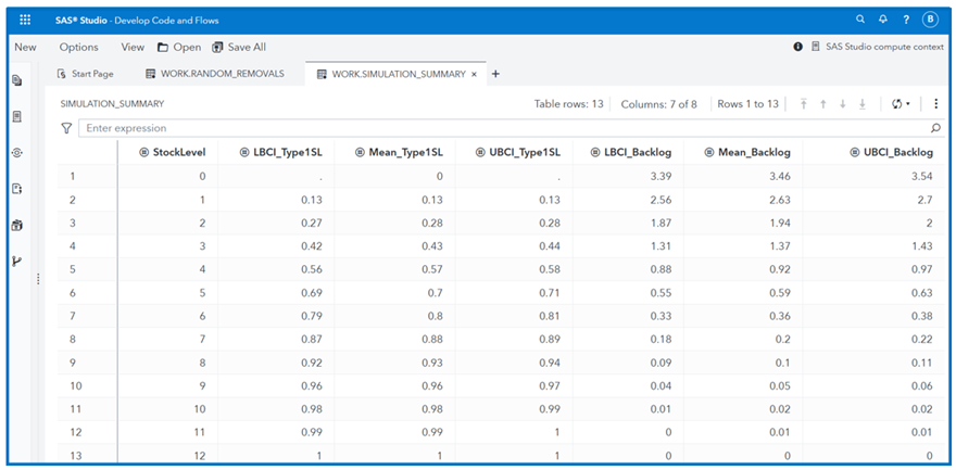
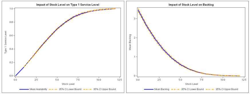
Figure 6 visualizes the results from Figure 5, showing how the mean Type 1 service and mean backlog vary with different inventory levels. The 95% confidence intervals, displayed to two decimal places, are relatively narrow, indicating low measurement error across 1,000 simulation replications.

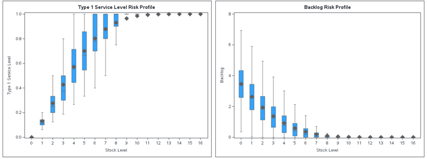
Figure 6: Sensitivity of mean type 1 service level and backlog to inventory levels

To gain a deeper insight into the variability and risk associated with availability and backlog, we use the same simulation output data to generate risk profiles, as shown in Figure 7. We illustrate each tested stock level by using a box-and-whisker plot.

Figure 7: Risk profiles for availability and backlog

Key takeaways: Smarter decisions through simulation

In summary, we have explained how to determine optimal spare parts inventory levels that minimize cost while meeting availability targets under uncertainty. At its core is a stochastic simulation. It predicts mean availability and backlog, along with their 95% confidence intervals and risk profiles, across various inventory levels. By combining stochastic simulation with SAS analytics, organizations can make data-driven decisions that balance cost, risk, and service levels. As a result, this approach enhances spare parts planning. Moreover, it enhances overall asset availability, particularly in environments where uptime is crucial.

Author Jagdishwar Mankala
Senior Data Scientist, SAS Pune Applied AI and Modeling

Jagdishwar Mankala is a Senior Data Scientist in the SAS Pune Applied AI and Modeling Division. He has over three years of experience specializing in optimization models, including inventory optimization and retail allocation. He holds a Master of Technology in Manufacturing Engineering from the Indian Institute of Technology (IIT) Bombay. Jagdishwar is passionate about leveraging data-driven insights to solve real-world challenges. Outside of work, he enjoys playing cricket, table tennis, and pencil sketching.

Author Jinxin Yi
Director, SAS Applied AI and Modeling

Jinxin Yi is a Director in the Applied AI and Modeling Division at SAS, where he leads teams of data scientists in developing analytical models for business applications. He holds a Ph.D. in Operations Research from Carnegie Mellon University.