Editor's note: this post was co-authored by Kevin Scott and David Frede.
Batch manufacturing involves producing goods in batches rather than in a continuous stream. This approach is common in industries such as pharmaceuticals, chemicals, and materials processing, where precise control over the production process is essential to ensure product quality and consistency. One critical aspect of batch manufacturing is the need to manage and understand inherent time delays that occur at various stages of the process.
In the glass manufacturing industry, which operates under the principles of batch manufacturing, precisely controlling the furnace temperature is essential for producing high-quality glass. The process involves melting raw materials like silica sand, soda ash, and limestone at high temperatures, where maintaining the correct temperature is crucial.
Scenario and Control Setting Change
When the quality control system detects suboptimal glass viscosity for the forming processes, adjustments to the kiln temperature are required to alter the glass’s viscosity. If the glass needs to be less viscous, the kiln’s temperature set point is increased accordingly.
Inherent Time Delays
This adjustment introduces several types of delays:
- Physical Delay: The furnace, with its massive firebrick linings and vast quantities of molten glass, exhibits significant thermal inertia, meaning it reacts slowly to changes in heating rates.
- Chemical Delay: The raw materials and the glass itself also take time to reach a new equilibrium state. Achieving a uniform temperature throughout the furnace, crucial for the materials to melt and homogenize properly, can take considerable time.
- Logistical Delay: Delays are further influenced by the positioning of temperature sensors and the distribution of heat sources within the furnace. Changes may not be immediately registered by sensors, especially if they are located far from direct heat adjustments.
Observable Effects and Process Impact
The desired change in viscosity will only become measurable hours later, once the entire system has adjusted to the new temperature settings. During this period, the furnace must be monitored to ensure the temperature stabilizes as intended, requiring operators to anticipate changes and act proactively.
Implications for Anomaly Detection
These inherent delays pose significant challenges when integrated into anomaly detection systems, which are crucial for ensuring continuous process quality and safety.
Problem Setup
- Delayed Series: This refers to the sensor data collected during the manufacturing process, which includes the described inherent delays.
- Golden Batch: This is the optimal dataset against which current production is compared to detect anomalies.
Anomaly Detection Challenges
Anomaly detection algorithms, sensitive to deviations in timing, data patterns, and other critical pa- rameters, might misinterpret the delayed sensor readings as anomalies if:
- The delayed response appears out of sync with the expected timeline and values of the golden batch, leading to false positives.
Example and Necessary Adjustments
For instance, if the anomaly detection system compares the temperature readings of a current batch, which exhibit delayed stabilization, against a golden batch that stabilized quicker, it could erroneously flag this as an anomaly. To avoid such errors:
- Time Shift Handling: Anomaly detection systems need to be designed with an awareness of these known delays. Preprocessing steps might detecting delays and then shifting the time series data of the delayed series to align with the golden batch timeline before analysis.
- Algorithm Configuration: Incorporating dynamic adjustments for expected delays within the anomaly detection algorithm itself can be crucial.
Cross-Correlation Analysis for Time Delay Detection
Given the challenges presented by inherent delays, we utilize cross-correlation analysis to detect time delays between the golden batch and a production batch affected by a logistical delay at the beginning of the heating process.
Golden Batch Heating Schedule
- Stage 1: Ramp up from room temperature (25°C) to 600°C at a rate of 150°C/hour.
- Stage 2: Hold at 600°C for 30 minutes.
- Stage 3: Ramp up from 600°C to 1200°C at a rate of 300°C/hour.
Production Delay Series
- Stage 0: 45 minute delay at the start.
- Stage 1: Ramp up from room temperature (25°C) to 600°C at the same rate as the golden batch.
- Stage 2: Same hold time at 600°C.
- Stage 3: Same ramp up rate to 1200°C.
The cross-correlation analysis will compare the temperature profiles from these two series to quantify the delay introduced by the logistical issues in the production batch. This analysis will help determine the extent to which the delay impacts the synchronization of process temperatures, which is critical for understanding potential deviations in product quality.
Data Simulation for Cross-Correlation Analysis
To illustrate this process, the following SAS DATA step simulates the temperature profiles of both the golden batch and the delayed production batch. The temperature profiles will then be used for cross- correlation analysis.
data viscosity_simulation; /* Constants for Log Viscosity Equation */ A = -2.585; B = 4215; T0 = 263; /* Define kiln heating stage durations in minutes */ stage_0_duration = 45; stage_1_duration = int((600 - 25) / (150 / 60)); stage_2_duration = 30; stage_3_duration = int((1200 - 600) / (300 / 60)); /* Total duration */ do series_id=1 to 2; if series_id=1 then total_duration = stage_1_duration + stage_2_duration + stage_3_duration; else total_duration = stage_0_duration + stage_1_duration + stage_2_duration + stage_3_duration; /* Initialize time and temperature arrays */ do time = 0 to total_duration; if series_id=1 then do; /* Define temperatures for each stage */ if time <= stage_1_duration then do; temperature_C = 25 + (150 / 60) * time + 4*RAND('NORMAL'); end; else if time <= stage_1_duration + stage_2_duration then do; temperature_C = 600 + 4*RAND('NORMAL'); end; else do; temperature_C = 600 + (300 / 60) * (time - stage_1_duration - ,→ stage_2_duration) + 4*RAND('NORMAL'); end; end; else do; /* Define temperatures for each stage */ if time <= stage_0_duration then do; temperature_C = 25 + 1*RAND('NORMAL'); end; else if time <= stage_0_duration + stage_1_duration then do; temperature_C = 25 + (150 / 60) * (time - stage_0_duration) + ,→ 4*RAND('NORMAL'); end; else if time <=stage_0_duration + stage_1_duration + stage_2_duration then ,→ do; temperature_C = 600 + 4*RAND('NORMAL'); end; else do; temperature_C = 600 + (300 / 60) * (time - stage_0_duration - ,→ stage_1_duration - stage_2_duration) + 4*RAND('NORMAL'); end; end; /* Calculate log viscosity */ log_viscosity = A + B / (temperature_C - T0); /* Output the values */ output; end; end; drop stage_0_duration stage_1_duration stage_2_duration stage_3_duration ,→ total_duration; run; data viscosity_simulation_goldbatch(where=(series_id=1) ,→ rename=(temperature_c=temperature_gb) keep=series_id time temperature_c) viscosity_simulation_delay(where=(series_id=2) ,→ rename=(temperature_c=temperature_d) keep=series_id time temperature_c); set viscosity_simulation; run; proc sort data=viscosity_simulation_goldbatch(drop=series_id); by time; run; proc sort data=viscosity_simulation_delay(drop=series_id); by time; run; data viscosity_simulation_both; merge viscosity_simulation_delay(in=a) viscosity_simulation_goldbatch(in=b); by time; run; |
Before performing the cross-correlation via PROC TIMESERIES we will use the following code to visualize the golden batch and delayed production batch.
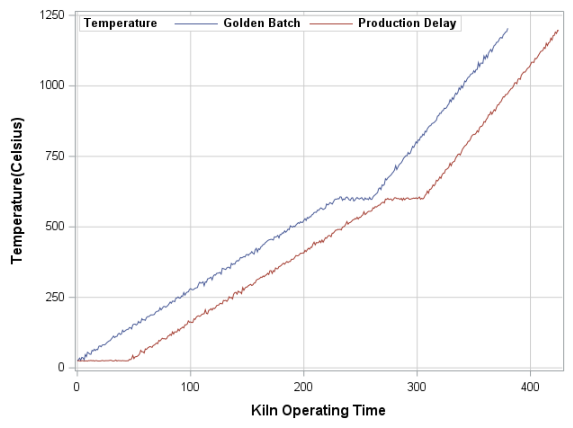
proc format; value MYfmt 1='Golden Batch' 2='Production Delay'; run; proc sgplot data=viscosity_simulation; format series_id MYfmt.; label temperature_C="Temperature(Celsius)" time="Kiln Operating Time"; styleattrs datacolors=(cxedf8fb cxb2e2e2 cx66c2a4 cx238b45 ); series x=time y=temperature_C / group=series_id name='series'; xaxis labelattrs=(size=12 weight=bold) valueattrs=(size=10) gridattrs=(color=graycc thickness=.25) grid; yaxis labelattrs=(size=12 weight=bold) valueattrs=(size=10) gridattrs=(color=graycc thickness=.25) grid; keylegend 'series'/ title="Temperature" titleattrs=(size=10 weight=Bold) valueattrs=(size=10 weight=Bold) location=inside position=nw across=2 opaque; run; |
Using the plot, we can confirm from the series plot that their is a delay in the production batch even though temperatures match the golden batch after the delay.
To identify the delay and post-process the production batch correctly so that it is not identified as an anomaly or outlier series we will identify the time delay using a cross-correlation analysis and visualize the the cross-correlation function for all lags between 0 and 60.
proc timeseries data=viscosity_simulation_both out=_NULL_ outcrosscorr=crosscorr; crosscorr _ALL_ / nlags=60; id time interval=day; var temperature_d temperature_gb; run; proc sgplot data=crosscorr(where=(lag>=0 and _name_="temperature_d")); series x=lag y=ccf / name='series'; xaxis labelattrs=(size=12 weight=bold) valueattrs=(size=10) gridattrs=(color=graycc thickness=.25) grid values=(5 15 25 35 45 55) valuesdisplay=('5' '15' '25' '35' '45' '55'); yaxis labelattrs=(size=12 weight=bold) valueattrs=(size=10) gridattrs=(color=graycc thickness=.25) grid; keylegend 'series' / title="CCF" titleattrs=(size=10 weight=Bold) valueattrs=(size=10 weight=Bold) location=inside position=nw across=2 opaque; refline 45 / axis=x label = ('45 Minutes') labelattrs=(size=10 weight=Bold) lineattrs=(thickness=1 color=black pattern=mediumdashdotdot ); run; |
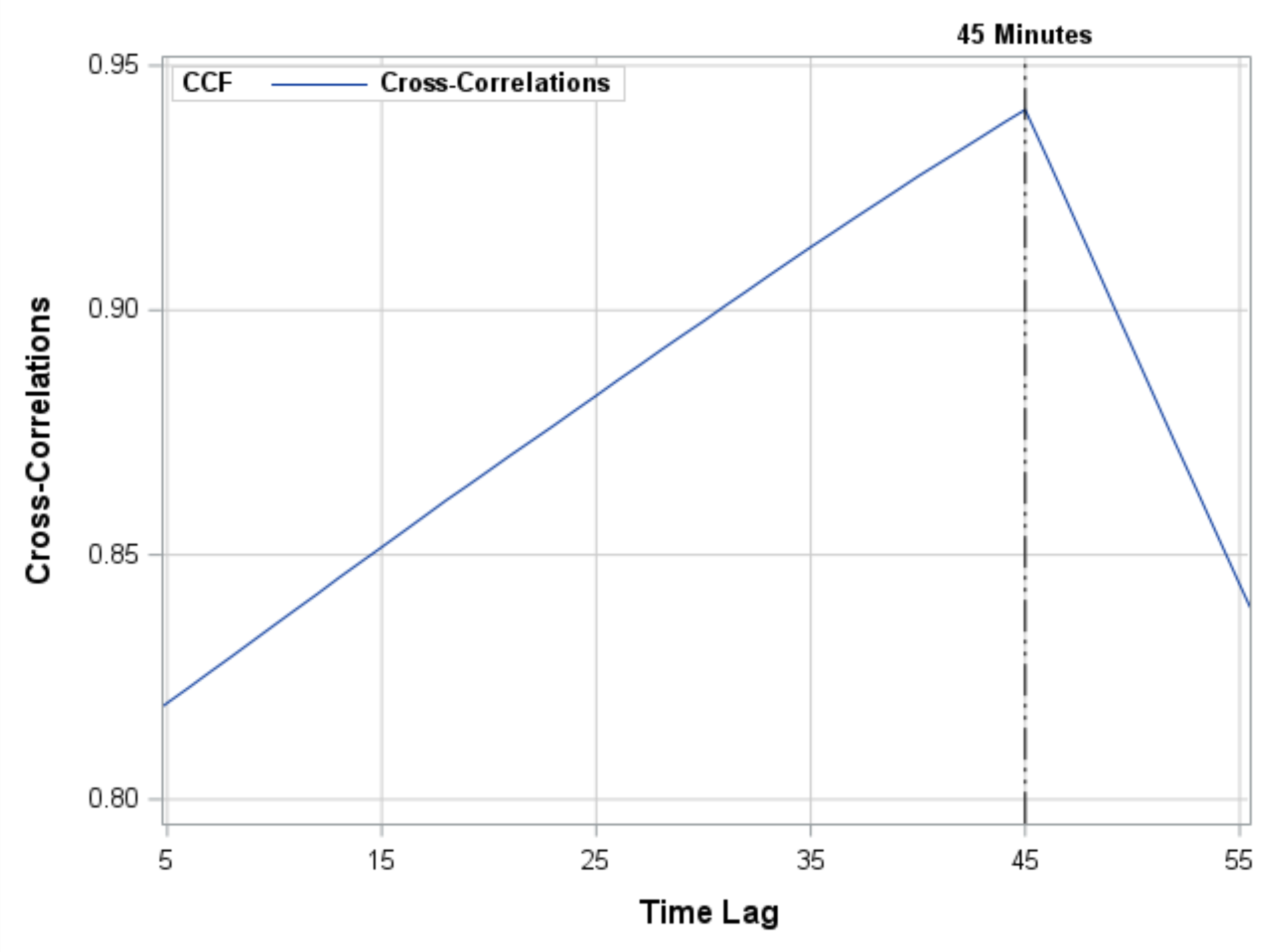
The plot of the cross-correlation function indicates the lag associated with the maximum cross- correlation is 45 minutes. The cross-correlation can be effective in identifying simple delays in batch production processes.
Series identified as time delays using cross-correlation analysis can be aligned using techniques such as dynamic time warping and sliding similarity analysis. These techniques are available within SAS/ETS in SAS 9.4 and Visual Forecasting in SAS Viya. The identification step reduces the number of series that must be warped and aligned, making the analytic processing more efficient.
Conclusion
Integrating domain knowledge about process dynamics and expected delays into the design and con- figuration of anomaly detection systems is beneficial and necessary. Properly handling time delays in anomaly detection is crucial for maintaining the reliability of monitoring systems, avoiding unnecessary alarms, and ensuring that manufacturing operations run smoothly and efficiently. This approach ensures accurate and relevant monitoring, safeguarding against the pitfalls of misinterpreting delayed responses as process failures or anomalies.