A crash course on deep learning in the cloud

Deep learning is the newest area of machine learning and has become ubiquitous in predictive modeling. The complex brain-like structure of deep learning models is used to find intricate patterns in large volumes of data. They have substantially improved the performance of general supervised models, time series, speech recognition, sentiment analysis. object detection, and image classification.

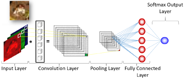
The image above displays the structure of a neural network used to classify a variety of different images. In this example, the red, green, and blue pixels of the frog image are passed to a convolutional layer to create model weights and a reduced representation of the pixels known as a feature map. The pooling layer then provides localized summaries of the feature maps and passes the information into a fully connected layer. This final layer uses the features extracted to predict the image category. If the model performs well, it should classify the image as a frog.

In my session at ODSC Europe, which inspired this post, participants experienced deep learning with SAS® Analytics and open source technologies, such as R and Python. Ever binge-watched films on Netflix? I also introduced students to factorization machines, which underlie uncannily precise movie recommendations. Read on to continue your crash course.

What is deep learning?

Deep learning is not simply a neural network with two or more hidden layers. The true essence of deep learning lies in the methods that enable the increased extraction of information derived from a neural network with more than one hidden layer. Adding more hidden layers to a neural network would provide little benefit without the methods that underpin the efficient extraction of information. Some of these methods are contrasted with their traditional counterparts below.

Traditional Neural Networks Vs Deep Learning
Hidden Activation Functions: Hyperbolic Tangent Vs Rectified Linear and others.
Weight Initialization: Constant Variance Vs Normalized Variance
Regularization: L1 and L2 Vs Dropout and Batch Normalization
Gradient-Based Learning: Batch Gradient Descent Vs Stochastic Gradient Descent
Processors: CPU Vs GPU

The use of rectified linear activation functions and normalized variance weight initialization help prevent neuron saturation. This occurs when the deep learning model parameters stop updating during the fitting process without having reached the optimal solution. Dropout and batch normalization are improved techniques that help prevent overfitting and improve generalizability. Stochastic gradient descent and GPUs improve the computational efficiency of deep learning models when the data becomes large or intractable.

Deep learning applications

The flexibility in deep learning models allows the practitioner to use different types of hidden layers to customize the neural network structure and analyze a variety of data. The traditional feed-forward neural network uses fully connected hidden layers to analyze static data to find nonlinear patterns. Recurrent neural networks use recurrent or gated hidden layers to model sequence data to account for the temporal structure. The introduction of gates in a recurrent neural network helps the model decide what information to move forward in time for prediction and what to disregard as irrelevant past information.

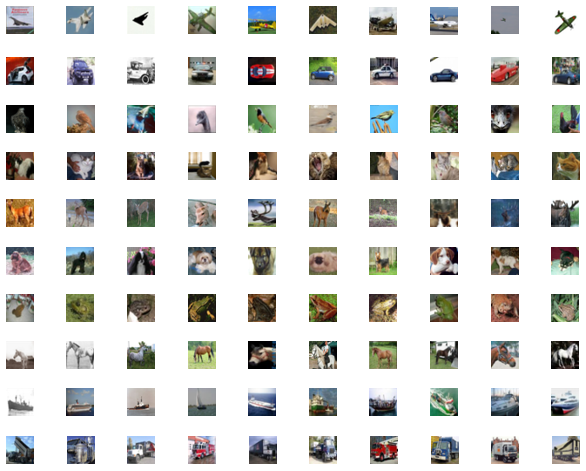
Convolutional neural networks use convolutional and pooling layers to learn from the pixels in the input images and help classify images into different target categories. The CIFAR-10 data set consists of 60,000 images and 10 classes (airplane, automobile, bird, cat, deer, dog, frog, horse, ship, and truck) and is commonly used to learn how to build a convolutional neural network and classify images.

Factorization machines

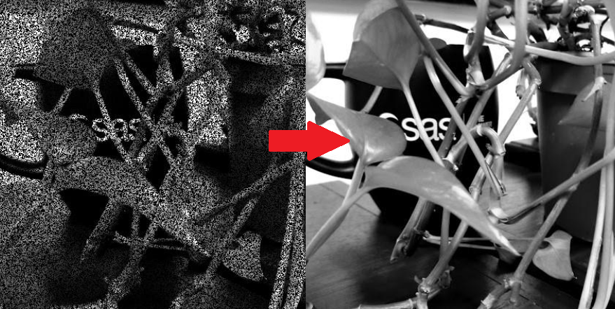
What happens when you have an incomplete image or a sparse matrix of pixels? How can you recover the image to view and interpret its original form? Factorization Machines are a relatively new and powerful tool for modeling high-dimensional and sparse data. Most commonly they are used as recommender systems by modeling the relationship between users and items.

For example, a factorization machine can be used to recommend your next Netflix binge based on how you and other streamers rate content. Factorization machines can also be used to impute missing pixels of a corrupted image to recover the original image. For example, historical art damaged in World War II can be restored to its original form using factorization machines.