Datasets are rarely ready for analysis, and one of the most prevalent problems is missing data. This post is the first in a short series focusing on how to think about missingness, how JMP13 can help us determine the scope of missing data in a given table, and how to address the problems that missing data can cause.

Will missing data be a problem in your study?

Whether or not missingness is a problem for a particular study depends on the analysis to be performed and the data types involved. Although each dataset can present unique issues, there are some common problems to anticipate. At the outset, it’s important to know that missing data can bias the conclusions of a study and/or distort estimates of variability. So, we don’t want to ignore what we cannot see.

If the number of missing cells is tiny in comparison to your entire sample, you might just forge ahead and omit the incomplete rows. If one column has many missing cells, you might similarly exclude that column from your models.

Blanks in one column are just part of the problem, because incompleteness in a row can knock the entire row out of a multivariate analysis. For example, suppose we intend to test a model with one response variable and three predictors. Many multivariable modeling methods require complete cases—so whenever a cell is blank, that row is dropped from the analysis. Hence, prevalence is not simply a question of counting the number of empty cells, but also recognizing how those missing observations are distributed through the data table.

How to hunt for missing data

As an example, consider the “Youth Risk Behavior Surveillance System” that generated the data found in the JMP13 Sample Data table titled Health Risk Survey. This particular iteration of the survey was taken in 2005, and researchers at the U.S. Centers for Disease control surveyed nearly 14,000 9th to 12th grade students about their health and behaviors. The main survey has nearly 100 questions, and respondents tend to answer most questions, but skip others.

Exploring this data table

The table has 204 columns and 13,917 rows. Within the Columns panel there are three sets of grouped columns, and I will work with the first group, which contain responses to the questions on the survey.

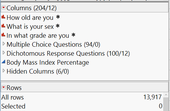
In this example, I’ll look at just 11 of the columns in this data table, and I intend to use “How often drive when drinking past 30 days” as the response variable (see below).

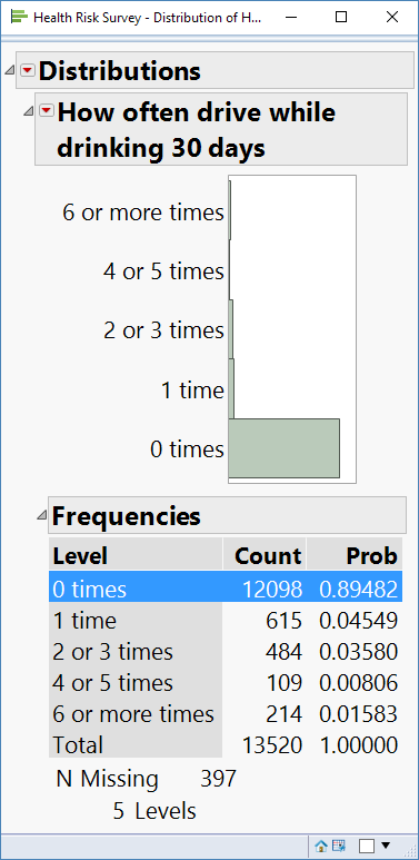
There are 397 missing values in this column, or approximately 3% of all respondents so any model we specify will begin with at most 97% of the rows in the sample. I now move on to seeing which combinations of potential predictor columns have missing data. Other things being equal, I’ll want a subset of columns that maximizes the useful sample size.

Choose Tables ► Missing Data Pattern.  In the Columns pane, click on the disclosure triangle next to Multiple Choice Questions. Select the 11 columns as shown here, then click Count Missing Value Codes and OK.

This aw generates a new table:

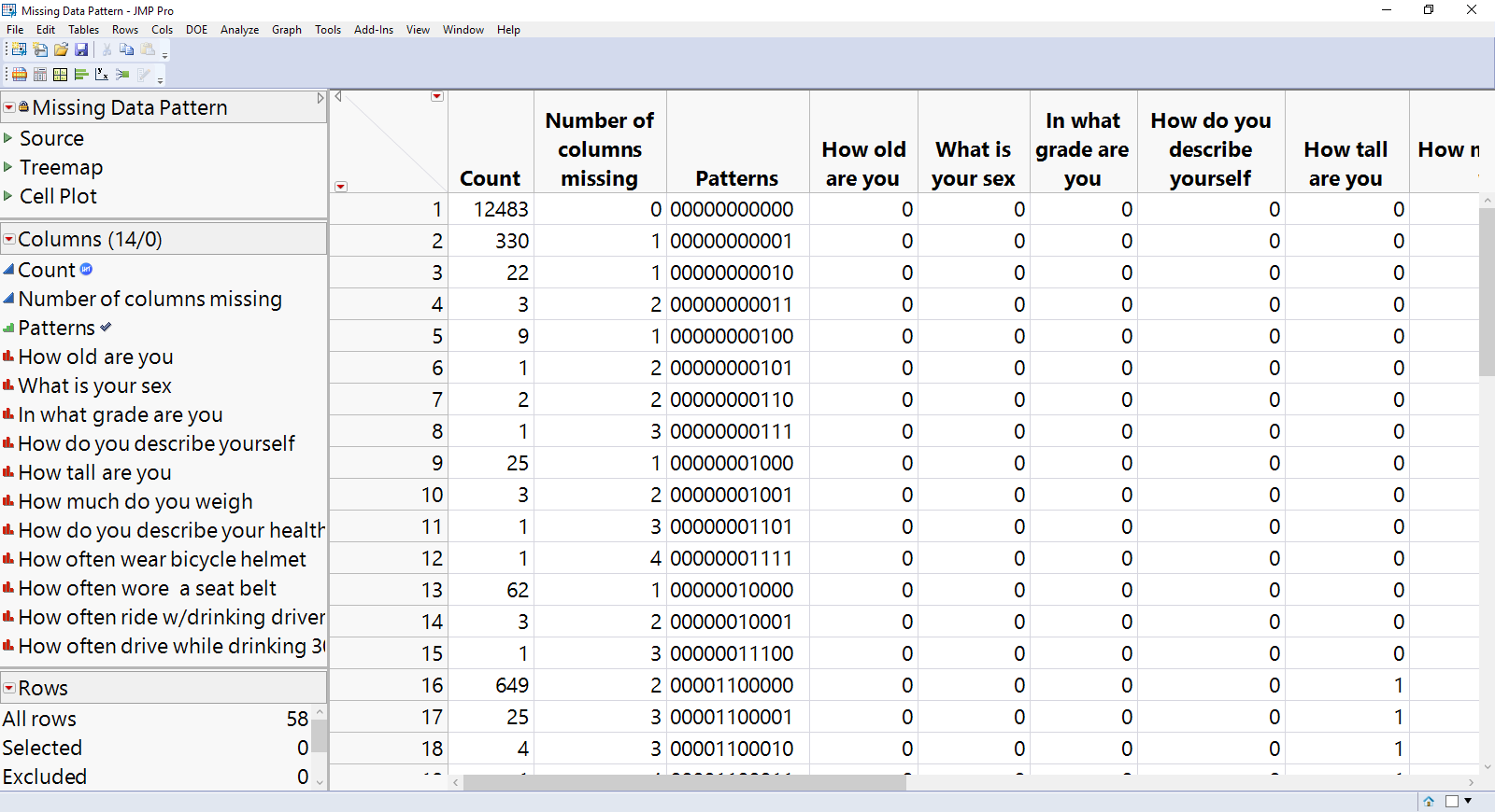
The first three columns of this table shows the frequency of each possible combination of missing cells across the selected columns. The remaining 11 columns have 0-1 indicators reflecting missingness. For example, row 1 of the table says that there 12,483 students who answered every question.

Row 2 shows that 330 students did not respond to our response variable (last column), but did answer all others. Wait a minute – earlier we saw that 397 answers were missing. What about the other 67? Those 67 are missing in combination with one or more other columns, as show in later rows with a 1 in the final position of the “Pattern”. The data table may be hard to scan visually, so JMP offers two visualizations of the patterns, generated by running the scripts in the table panel. Just click the green arrows next to Treemap and Cell Plot to investigate, but let’s look closely at the Cell plot, shown here:

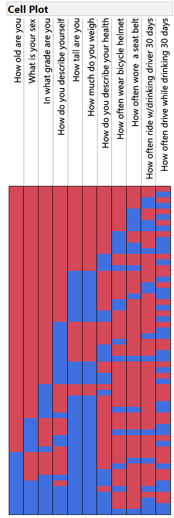
The right-most column is the response variable, and we see many blue cells where missing data occur. Look horizontally across the plot and contrast columns with red-blue pattern is similar to the response column. Those variables have little impact on the total usable sample size. However, if you try to include columns with blue cells where the response has red cells, the number of missing rows will begin to climb, as the Count column in the Missing Data table reveals.

This technique is one aspect of dealing with missing data illustrated in my new book Preparing Data for Analysis with JMP. It is also part of the larger process of mitigating the problems of missing observations. In my next post, I’ll look at common causes of missing data.