While many analysts understand how to interpret the parameter estimates from linear regression with continuous input variables, they may feel less comfortable with parameter estimates from models with categorical inputs. SAS modeling procedures (such as PROC REG and others) need numerical information to represent all inputs—including classification variables. Suppose we want to model the average amount spent on a credit card (SPEND) as a function of the variable INCOME (which has three levels: Low, Medium, and High). The words ‘Low’, ‘Medium’, and ‘High’ are meaningless to PROC REG and need to be translated into numbers. Many ways to represent these words as numbers exist.

One of the simplest coding schemes is GLM coding. It uses 0’s and 1’s instead of ‘Low’, ‘Medium’, and ‘High’. We replace the variable INCOME with three new variables, called ‘Design Variables’, ‘Dummy Variables’, or ‘Indicator Variables’; there will be one new design variable for each level of income.

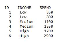
To be concrete, consider a very small data set with 6 observations: two observations for each level of INCOME:

Using a data step, add the three design variables (Low, Medium, and High) to the data set:

data spend2;
 set spend1;
 Low=(income='Low');
 Medium=(income='Medium');
 High=(income='High');
run;

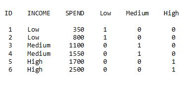
Note that the design variable for LOW has a value of 1 for observations with INCOME=Low and 0 for all other observations. A similar pattern is used for the design variables for Medium and High. When writing the PROC REG code for the model, use the design variables instead of the original variable INCOME:

proc reg data=spend2;
  model spend=low medium high;
run;

How do we interpret these parameters?  The note at the top, ‘high=Intercept-low-medium’ gives us a clue. It may not be obvious, but this means that the Parameter Estimate for the Intercept (2100) is the average SPEND amount when income is at the High level. High is the ‘Reference level’ for obtaining the average SPEND amounts for Low and Medium incomes. The parameter estimates for Low and Medium indicate how much above (for a positive parameter) or below (for a negative parameter) the average SPEND amount is for observations in these categories, as compared to the average SPEND amount for the reference level of High.

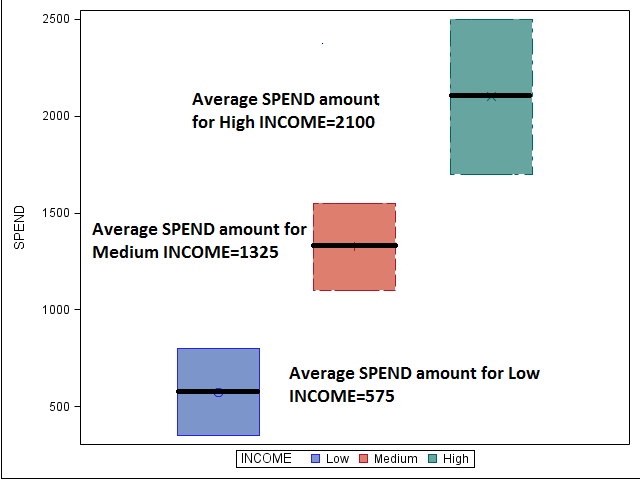
For Low income, the average SPEND amount is 2100-1525=575. For Medium income, the average SPEND amount is 2100-775=1325. To summarize, the average SPEND amounts are 575, 1325 and 2100 for income categories, low, medium, and high, respectively (shown in the boxplots below):

Why did we get that note at the top of the PROC REG output that read: ‘high=Intercept-low-medium’? Because we included all three design variables in our model. Once we identify which observations fall into the Low and Medium categories, it’s easy to figure out which are in the High category—all the leftovers. Putting all three design variables on the MODEL statement ‘overparameterizes’ the model, meaning we are providing information that SAS doesn’t really need; so it ignores the last level during estimation. For this reason, we only need to put two of the three design variables into our code.

proc reg data=spend2;
  model spend=low medium;
run;

By leaving High off the MODEL statement, we are making it the reference level. When we omit a level as shown here, the coding scheme is called ‘Reference Cell Coding’; the excluded level will be the reference level.

We can choose to have another reference level, by putting either Low or Medium last on the MODEL statement (or excluding one of them from the statement). The parameter estimates will change, but the average spend amounts will be the same. We'll illustrate this in the second installment of 'Those Pesky CLASS Variables.