Depending on who you talk to, you'll get varying definitions and opinions regarding demand sensing. Anything from sensing short-range replenishment based on sales orders, to the manual blending of point-of-sales (POS) data and shipments. But a key component for retailers and CPG companies is accurately forecasting short-term consumer demand to ensure that their products are available to consumers when they need them.
Implementing a short-term (one to eight week) forecast is critical to understanding and predicting changing consumer demand patterns associated with sales promotions, events, weather conditions, natural disasters and other unexpected shifts (anomalies) in consumer demand. Short-term demand sensing allows retailers and CPG companies to predict and adapt to those changing consumer demand patterns.
Key benefits for demand sensing
Traditional time-series forecasting techniques that model patterns associated with trend and seasonality are typically used for demand forecasting by retailers and CPG companies. These models can only uncover two historical demand patterns (trend and seasonality) and provide an estimate of demand into the future. In addition to the historical demand data, CPG companies have access to other data feeds like POS information, future firm open orders, promotional events, trade inventory and others that collectively constitute the demand and supply signals.
SAS® already provides the statistical engine that drives demand forecasting at several large retail and CPG companies. Those companies can use SAS to improve short-term demand sensing by augmenting traditional time-series forecasting with machine learning techniques and by incorporating additional demand signal data. The key benefits for using demand sensing include:
- Increase in sales revenue by improving sensing capability to drive an agile supply chain response to meet customer and consumer demand needs.
- Improvement in transportation planning with preferred carriers, reduction in execution costs by reducing redeployment and lowering inventory carrying costs.
- Improvement of customer service and on-shelf availability of products, ensuring consumers find the products they want and need.
- Improved revenue/profit through enhanced replenishment efficiencies and fewer stock-outs on shelf.
SAS now has a patent-pending machine learning (ML) approach to creating one-to-eight week – weekly and daily – demand forecasts. This new approach, combining segmentation analysis, machine learning and traditional time-series forecasting models, allows CPG companies to generate the improved forecasts by using historical supply signal (shipments) data in combination with point-of-sale data (demand signal), sales promotions, trade inventory and others.
A real-world example of demand sensing using machine learning
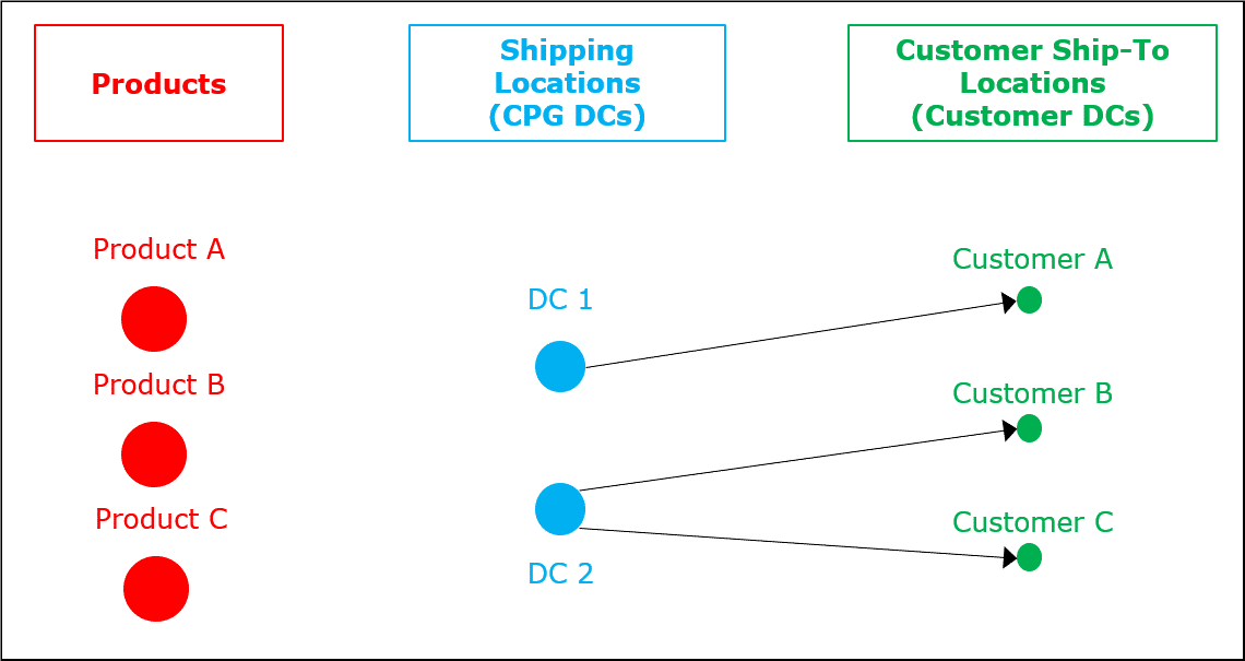
A large global CPG company provided us with seven years of order shipment history for triplets of Product (Prod=SKU), Shipping Location (ShipLoc) and Customer Location (CustLoc) at a weekly and daily resolution as shown in Figure 1.
Shipping locations corresponded to the CPG distributions centers (DCs) and retail customer locations were customer DCs. Thus, the order history corresponded to the number of daily product shipments from ShipLoc to CustLoc. We were also provided future open orders for both datasets at the lowest (Prod – ShipLoc – CustLoc) level. The shipment order history and future open orders were the main inputs in our forecasting advanced analytics models. We were provided with point-of-sale (POS) data and trade inventory data (Prod – ShipLoc – CustLoc = customer) for less than one year of history. See Figure 1.
In addition to the order history, future open orders and POS data, the customer provided weekly estimated forecasts using their current forecasting procedures and technology. Two such forecast estimates were provided. One was generated using standard procedures based on SAS (FC-Base), and another was generated by experts who adjusted FC-Base to further refine the existing forecasts (FC-Base+Expert). Each of these forecast estimates were provided at the (Prod) and (Prod – ShipLoc) levels.
The main goal of this project was to generate better forecast estimates compared to FC-Base and FC-Base+Expert at both (Prod) and (Prod – ShipLoc) levels. Note that the forecasts for comparison were only provided at the weekly level. The CPG company did not provide daily forecasts for comparison--they currently do not have the capability to forecast daily.
Rolling weekly forecasts
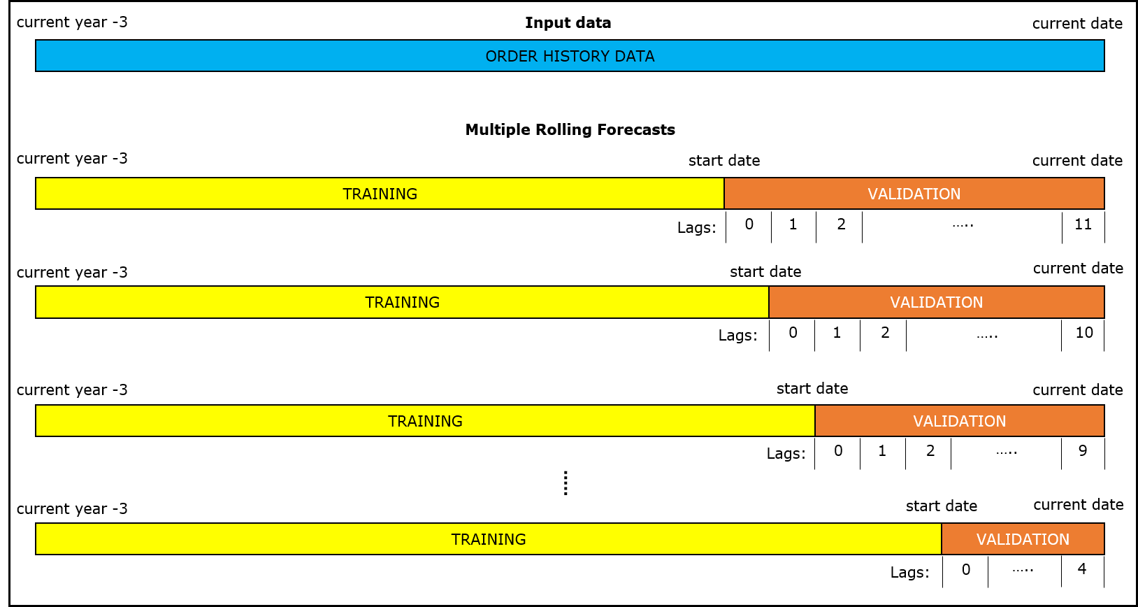
Several rolling weekly forecasts for different forecast starting dates were generated. Order history data prior to a given forecast start date was used for training, and 12 weeks of data after the start date was used as the holdout data for validation (demonstrated in Figure 2). For each rolling forecast, we compared performance for the current week (Lag 0) and up to twelve weeks into the future (Lag 11).
For each rolling forecast, we used two methods to generate forecasts:
- Traditional time-series based forecast.
- Neural Network + Time-Series (NNTS) forecast.
For the time-series based forecast, the SAS traditional times series forecasts are used to diagnose the statistical characteristics of each {Prod – ShipLoc – CustLoc} triplet time series and identify appropriate forecasting models for each data set. The diagnosis of the results was used to generate a time-series forecast estimate and a trend estimate for each {Prod – ShipLoc – CustLoc} triplet.
Results
We generated enhanced weekly and daily forecasts for the products that passed our data validation criteria, that is, order shipments in the current year and at least one year of order history. The performance of weekly and daily forecasts was evaluated using two metrics:
- Accuracy, which considers the absolute error between the forecasted order quantity and the actual order quantity.
- Bias, which considers the ratio between the actual order quantity and the forecasted order quantity. A negative bias is interpreted as an under-forecast of the actual quantity, whereas a positive bias is interpreted as an over-forecast of the actual order quantity.
For weekly forecasts, we evaluated the above measures for our enhanced forecast (FC-Enhanced) and the two forecasts provided by the CPG company--FC-Base and FC-Base+Expert at both {Prod} and {Prod – ShipLoc} levels.
Weekly/daily forecast comparisons
Reviewing the results at the Material level, we can see in Figure 3 that the blue line indicates FC-Base forecast, the orange line indicates the FC-Base+Expert forecast and the grey line indicates combined enhanced machine learning and times series forecast. As you can see, the enhanced forecast is consistently more accurate than both CDP and Stat forecast. The CDP forecast is what is currently used in supply chain operations as the demand plan.
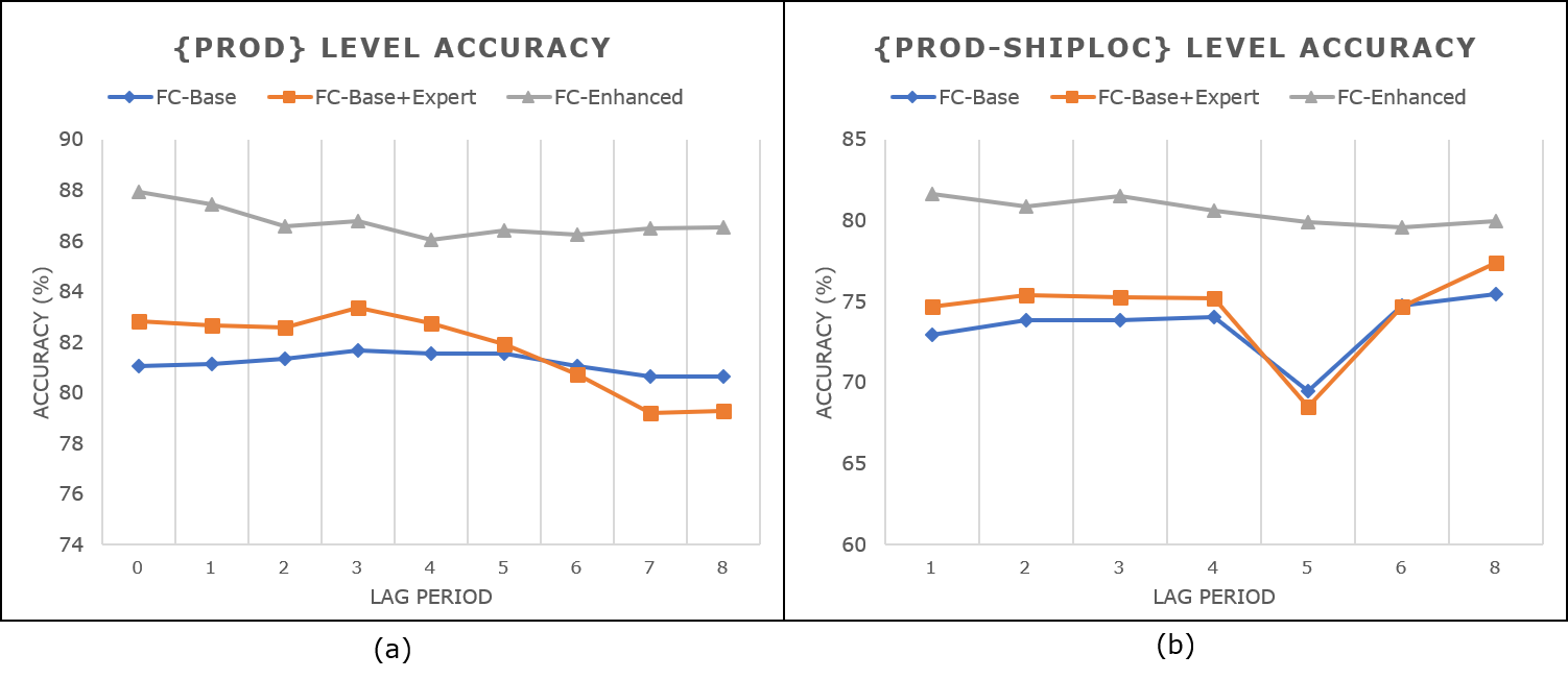
The bar chart at the top shows the enhanced forecast accuracy improvement over the FC-Base+Expert forecast. The enhanced forecast is 4% to 5% more accurate in the short term and around 7% to 9% between weekly lag periods six and eight. The results at Prod-SHipLoc level, we see similar trends to the Prod level. The enhanced forecast is 4% to 14% better than the FC-Base+Expert forecast.
After generating weekly forecasts, we separated them into daily forecasts based on long-term seasonality, short-term trends and non-linear trends using machine learning. See Figure 4.
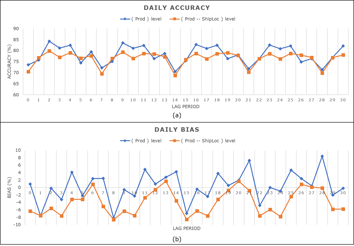
We observed that our average weekly forecast accuracy is 81.6% over eight-week lag periods. After disaggregating weekly forecasts to daily forecasts, we get an average accuracy of 73.8% over thirty daily lag periods. There was an average drop of 7.8% when disaggregating weekly forecasts to daily forecasts. The daily forecast accuracy is relatively stable across the thirty daily lag periods.
The bottom line
The use of machine learning clearly demonstrates how this patent-pending technique can be used effectively to enhance weekly and daily product demand forecasts. This new weekly forecasting methodology uses a combination of traditional time-series models and machine learning methods to automatically choose the best model for each {Prod – ShipLoc – CustLoc} combination. This new approach using machine learning establishes the efficacy of these methods by improving short-term forecasts for a large CPG company. At the weekly and daily level, there was a significant improvement in forecast accuracy over existing forecasting procedures across multiple lag periods.
The results also demonstrate that point-of-sale and customer inventory data further improves the daily and weekly forecast accuracy. We believe that our methods provide a flexible, transparent and scalable solution for effective supply chain management for CPG companies, which can also be utilized by retailers.
Learn more by downloading the white paper, Using Machine Learning and Demand Sensing to Enhance Short-Term Forecasting.