Peg solitaire

I love puzzles; I have a few of them in my office. I regularly use them at interviews: I ask the candidate either to solve a puzzle or to devise a (clever) mathematical algorithm that solves it.

I'm sure a lot of readers are familiar with the standard peg solitaire. You probably have one in your game room or bought one for your kids at some point. The goal in these games is to eliminate pegs by jumping over them with existing pegs until there is only one peg left, preferably in a predefined position. One difficulty with these games is that due to the large number of pegs it is very hard to think about a solution strategically from the beginning of the game. That is why they tend to just collect dust.

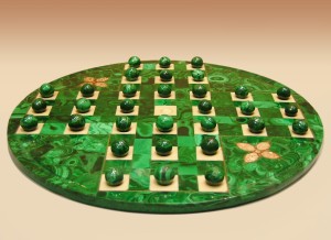
A friend of mine developed a different version, played on the following pentagonal board (see his blog post in Hungarian here):

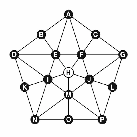
The goal is the same: initially the board is full and only the middle cell is empty. You can jump over one peg, land on the immediately following cell, and remove the peg you jumped over. The goal is to eliminate all but one peg, with the last peg ending up in the middle.

Modelling the puzzle

I thought to take the opportunity to solve this puzzle using SAS/OR optimization tools, in particular PROC OPTMODEL and the mixed integer linear programming (MILP) solver.

The entire PROC OPTMODEL code with comments is at the end of this post. There are a few points that I would like to elaborate on.

The board

The position of the board is represented by 16 binary variables after each round: board[i,j] = 1 if in round i a piece is placed in cell j, and 0 otherwise. At every move we change exactly three of these variables: two will go from 1 to 0, and one will go from 0 to 1. So we need to generate the possible differences between two consecutive rounds.

The moves

It turns out that there are 40 possible moves: we store 20 of them in a data set, the other 20 are just the reverse moves. A set of binary variables for each possible move in each round identifies which move was taken. In each round we can take exactly one move.

Strengthening the formulation

We added an extra constraint on the number of pegs on the board after each move. This is not necessary, but it helps to solve the problem faster. Strengthening optimization problem formulations this way is the key to solving a lot of practical problems.

Solving the puzzle

Then all we need to do is define the start and end positions and call the solver.

When the solution is returned we want to print it using the original labelling. Here we need to be careful: when we are checking which variables are 1 (so that we know which move was taken) we cannot simply check for equality, because optimization solvers use a nonzero feasibility tolerance. So even if we restrict a variable to be either 0 or 1, values within $10^{-6}$ of either value are still allowed. Thus we compare the solution values to 0.5 to decide if they are 0 or 1.

Finally, it is obvious from the board that there are many symmetric solutions. This is also clear from the solver log: our MILP solver takes this into account automatically, and eliminates the symmetric solutions from the search tree.

Variations and a conjecture

Having this code also makes it possible to analyze the game a bit. A natural question is: which start/end combinations are possible? It turns out that if the original empty cell is in the inside pentagon (E, F, J, M, I, H), then the final cell can be anywhere in the inside pentagon. Similarly, if the starting empty cell is on the outside (A, C, G, L, P, O, N, K, D, B), then the last peg remaining can be anywhere on the outside. But I couldn't solve any instance of the problem where this is not the case. That got me thinking if it was possible to have the initial empty cell inside and the final peg outside, and found a proof that it was not possible. (The proof is left as an exercise for the reader.)

Other ways to solve the problem

One could model the problem using constraint programming now that it is available through PROC OPTMODEL (as of version 13.2 of SAS/OR).

Another alternative is to create a large directed graph where each node of the graph is a possible state of the board, and the directed edges point to a node if it can be reached from a given node. Since there are only 16 cells in the original board, there are only $2^{16}=65536$ nodes in the graph. Then PROC OPTNET or the network solver in PROC OPTMODEL can be used to find which nodes are reachable from a given node. This way the complete game (every starting and ending position) can be analyzed easily.

PROC OPTMODEL code

Here is the entire code. Running it for the original problem takes less than a second using SAS/OR 13.2.

Special thanks to Rob Pratt for his help with the OPTMODEL code.

/* this is a data set of possible (half)moves */
data moves;
   input from $ take $ to $;
	datalines;
H M O 
H I K 
H E B 
H F C 
H J L 
M I D 
M J G 
I M P 
I E A 
E I N 
E F G 
F E D 
F J P 
J M N 
J F A 
N K D 
N O P 
D B A 
A C G 
G L P 
;
proc optmodel;
   /*let us fill up the entire board with 0 and 1*/
   set CELLS = /A B C D E F G H I J K L M N O P/;
   num boardstart{CELLS} init 1;
   num boardend{CELLS}   init 0;
 
   /* the status of the board before a round*/
   /* a binary variable for each cell*/
   /* 1 if there is a piece there, */
   /* 0 if the square is empty*/
   num numrounds = 14;
   set ROUNDS = 0..numrounds;
   var board{ROUNDS, CELLS} binary;
 
   /* a binary variable for all 40 possible moves in each round*/
   set OBS;
   set MOVES init OBS;
   var move{ROUNDS diff {numrounds}, MOVES} binary;
 
   /* a data matrix on what each move is*/
   /* this will be filled in later*/
   num edge{CELLS, MOVES} init 0;
 
   /* where a move starts*/
   str from{MOVES};
 
   /* which cell does a move take*/
   str take{MOVES};
 
   /* where a move ends*/
   str to{MOVES};
 
   /* read the three columns into our arrays*/
   read data moves into OBS=[_N_] from take to;
 
   /* double these to get all the possible moves*/
   num cardOBS = card(OBS);
   MOVES = 1..2*cardOBS;
   for {i in OBS} do;
      from[i+cardOBS] = to[i];
      to[i+cardOBS]   = from[i];
      take[i+cardOBS] = take[i];
   end;
 
   /* now let us fill in the edge matrix;*/
   /* for any (from take to) triplet we have*/
   /* edge[from,move] = -1*/
   /* edge[take,move] = -1*/
   /* edge[to,move] = +1;*/
   for {i in MOVES} do;
      edge[from[i],i] = -1;
      edge[take[i],i] = -1;
      edge[to[i],i]   =  1;
   end;
 
   /* starting position;*/
   con startcon{i in CELLS} : board[0,i] = boardstart[i];
 
   /* final position;*/
   con endcon{i in CELLS} : board[numrounds,i] = boardend[i];
 
   /* in each round the board can change */
   /* by one of the column vectors in the edge matrix;*/
   con round{i in ROUNDS diff {numrounds}, j in CELLS} :
      board[i+1, j] - board[i,j] = sum{k in MOVES} edge[j,k] * move[i,k];
 
   /* one move in each round;*/
   con onemove{i in ROUNDS diff {numrounds}} : 
      sum{k in MOVES} move[i,k] = 1;
 
   /* set the number of pieces on the board*/
   /* this makes the problem easier;*/
   con number{i in ROUNDS} : 
      sum{j in CELLS} board[i,j] = card(CELLS)-1-i;
 
   /* specify the starting and ending position*/
   /* at the beginning, cell START is empty*/
   /* at the end, cell END has the last piece;*/
   str START = 'H';
   str END   = 'H';
   boardstart[START] = 0;
   boardend[END] = 1;
 
   min Zero = 0; /* objective is optional in 13.2 */
 
   /* let us solve the problem;*/
   solve;
 
   /* create the solution table;*/
   str solution{ROUNDS diff {numrounds}, 1..3};
   for {i in ROUNDS diff {numrounds}} do;
      for {j in MOVES: move[i,j] > 0.5} do;
	solution[i,1] = from[j];
	solution[i,2] = take[j];
	solution[i,3] = to[j];
	leave;
      end;
   end;	
 
   print solution;
quit;

This is the output from SAS/OR:

NOTE: Problem generation will use 4 threads.
NOTE: The problem has 800 variables (0 free, 0 fixed).
NOTE: The problem has 800 binary and 0 integer variables.
NOTE: The problem has 285 linear constraints (0 LE, 285 EQ, 0 GE, 0 range).
NOTE: The problem has 2960 linear constraint coefficients.
NOTE: The problem has 0 nonlinear constraints (0 LE, 0 EQ, 0 GE, 0 range).
NOTE: The OPTMODEL presolver is disabled for linear problems.
NOTE: The MILP presolver value AUTOMATIC is applied.
NOTE: The MILP presolver removed 216 variables and 80 constraints.
NOTE: The MILP presolver removed 788 constraint coefficients.
NOTE: The MILP presolver modified 0 constraint coefficients.
NOTE: The presolved problem has 584 variables, 205 constraints, and 2172 constraint coefficients.
NOTE: The MILP solver is called.
          Node  Active    Sols    BestInteger      BestBound      Gap    Time
             0       1       0              .              0        .       0
NOTE: The MILP solver's symmetry detection found 92 orbits. The largest orbit contains 10 variables.
             0       1       0              .              0        .       0
           100       6       0              .              0        .       0
           200       5       0              .              0        .       0
           234       7       1              0              0    0.00%       0
NOTE: Optimal.
NOTE: Objective = 0.

NOTE: PROCEDURE OPTMODEL used (Total process time):
      real time           0.57 seconds
      cpu time            0.57 seconds

And a solution for the original problem (initial empty cell in the middle, final peg also in the middle):

   1 2 3 
 0 B E H 
 1 G F E 
 2 P L G 
 3 H E B 
 4 N I E 
 5 D K N 
 6 A B D 
 7 G C A 
 8 A E I 
 9 O M H 
10 D I M 
11 H J L 
12 N M J 
13 L J H