It is January. In the United States, this means NFL playoff time! A perfect time (if you are a geeky SAS/OR guy) to use PROC OPTGRAPH to rank the best teams in the NFL.

Ranking Sports Teams

Ranking of sports teams is a popular (and controversial) topic, especially in the world of college football, where from 1998 to 2013, rank determined a team's ability to play for the title (the BCS rankings). NFL rankings do not determine anything (as it should be) and are only for fun. This blog post attempts to see if an analytical ranking method (based purely on simple statistics and some linear algebra) can come close to the rankings determined by a panel of experts--for the NFL, that is the ESPN Power Rankings.

The motivation for this approach came from the excellent SAS Global Forum 2008 paper Generalizing Google’s PageRank to Rank National Football League Teams by Govan, Meyer, and Albright. In this paper, the authors present several different methods for ranking NFL teams by using PROC IML. We will focus on the Keener approach to ranking teams, as presented in The Perron-Frobenius Theorem and the Ranking of Football Teams.

The Keener Score

The main idea of the paper is that one can formulate a relationship $a_{ij}$ between teams $i$ and $j$ based on information gained from previous games. These relationships form an asymmetric matrix $A$ (imagine one row and one column for each team). The value $a_{ij}$ is a relative measure of how well team $i$ played against team $j$, while $a_{ji}$ is a measure of how well team $j$ played against team $i$. From this matrix, Keener proceeds to explain how the strength (or rank) of a team can be determined by finding the dominant eigenvector of matrix $A$. The dominant eigenvector is the eigenvector associated with the largest eigenvalue. Notice that, under some technical conditions, the Perron-Frobenius theorem ensures that the dominant eigenvector is unique and has strictly positive entries.

That is pretty cool! Does that really work? We'll check on that later. So far, we have considered only the math. But what about the data? What data should we use to define the relationship values $a_{ij}$ ? Here is where the art comes into play.

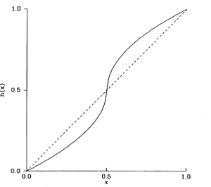
The most straightforward and obvious approach is to let $a_{ij}=s_{ij}$ be the number of points scored by team $i$ on team $j$ over the course of the season. However, as Keener points out, this approach is too naive. For example, using scores directly, the algorithm is susceptible to manipulation since teams can affect their ranking by running up scores (scoring far more points than needed to win a game). To combat this, Keener suggests the following nonlinear scoring function:

$\begin{align*} a_{ij} &= h \left( \frac{s_{ij} + 1}{s_{ij} + s_{ji} + 2} \right)\\ h(x) &= \frac{1}{2} + \frac{1}{2} sgn \left( x-\frac{1}{2} \right) \sqrt{|2x-1|} \end{align*}$

Applying this function awards teams for winning but is not as greatly influenced by running the score up. The function $h(x)$ is continuous, awards $0.5$ for a tie when $s_{ij}=s_{ji}$, and goes rapidly to $0$ or $1$.

Eigenvector Centrality in PROC OPTGRAPH

The mapping between a matrix and a directed graph here should be obvious. A link from node $i$ to node $j$ in the directed graph represents a game played between teams $i$ and $j$. The weight of the forward link from $i$ to $j$ gives the points scored by team $i$ on $j$. The reverse link (from $j$ to $i$) gives the converse.

The data for the points scored during the regular season can be found in a nice CSV format here.

I have imported this into a SAS data set nfl2014 and constructed the Keener score link weights with the following code: Now we have a directed graph where the weights of the links represent the Keener score. The OPTGRAPH procedure provides a number of metrics for measuring the importance of nodes in a graph. In the area of Social Network Analysis these are called centrality measures. Refer to the OPTGRAPH documentation for more information. In this particular case, we are dealing with a directed graph, so we need to use the power method (centrality eigen_algorithm=power option). 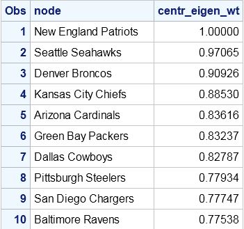The resulting ranking is now stored in the data set nfl2014Ranking17.

Comparing to ESPN's Power Rankings

The ESPN Power Rankings are determined by a poll of expert sports analysts. It is not clear if these analysts use any actual analytics, but I thought it would be interesting to compare our results using Keener's method with PROC OPTGRAPH.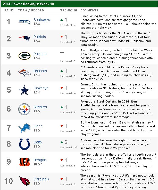 Surprisingly, the results are not that far off! The results by OPTGRAPH and ESPN have seven of the top ten teams in common. They both pick Seattle and New England as 1 and 2 (although they disagree on which team should be number 1). Considering we used only points scored to do the analysis, this is very interesting. Of course, the ESPN experts are using a huge amount of human intelligence to make their rankings, as well as using a poll of perhaps differing opinions. This has pros and cons over the purely analytic approach. The con of ESPN's approach is, obviously, that emotion comes into play. The experts are still human, and humans are inherently emotional and easily biased. The purely analytic approach will give you the mathematically correct answer, but this makes the assumption that your metric (the Keener score) is appropriate and comprehensive.

Let's consider one specific difference in the resulting rankings - the Kansas City Chiefs. In the OPTGRAPH rankings, they are the 4th best team, but ESPN has them the 13th best. Conversely, ESPN has the Detroit Lions as the 7th best team, while OPTGRAPH ranks them the 16th best team. The Chiefs ended the season 9-7, while the Lions ended the season 11-5. So, how did OPTGRAPH conclude that the Chiefs should be ranked higher than the Lions?

The reasoning is quite clear when you focus in on the schedules of the teams played by the Chiefs. The Chiefs played six teams which are ranked in the top ten (including the number 1 and 2 ranked teams), while the Lions played only three top-ranked teams. This is one of the key elements of the Keener approach using the dominant eigenvector. The strength of the schedule plays a large role in determining rank. This is clearly a controversial approach to ranking systems, and the experts at ESPN don't exactly agree. What do you think?

Acknowledgement: Rob Pratt

License Note: PROC OPTGRAPH requires a Social Network Analysis license. It is not included with a SAS/OR license, although it is developed and supported in the same department that works on SAS/OR.