This is the 12th installment of the "Getting Started" series. Furthermore, this is the third of three posts about the three statements that you can use in PROC SGPLOT that fit regression functions: REG, PBSPLINE, and LOESS.

Loess is a statistical methodology that performs locally weighted scatter plot smoothing. Loess provides the nonparametric method for estimating regression surfaces that was pioneered by William S. Cleveland and colleagues. The methodology behind the LOESS statement, like the PBSPLINE statement (and unlike the REG statement), makes no assumptions about the parametric form of the regression function. The LOESS statement provides some of the same methods that are available in PROC LOESS.

The LOESS statement fits loess models, displays the fit function(s), and optionally displays the data values. You can fit a wide variety of curves. You can fit a single function, or when you have a group or classification variable, fit multiple functions. (PROC SGPLOT provides a GROUP= option whereas statistical procedures usually provide a CLASS statement that you can use to specify groups.)

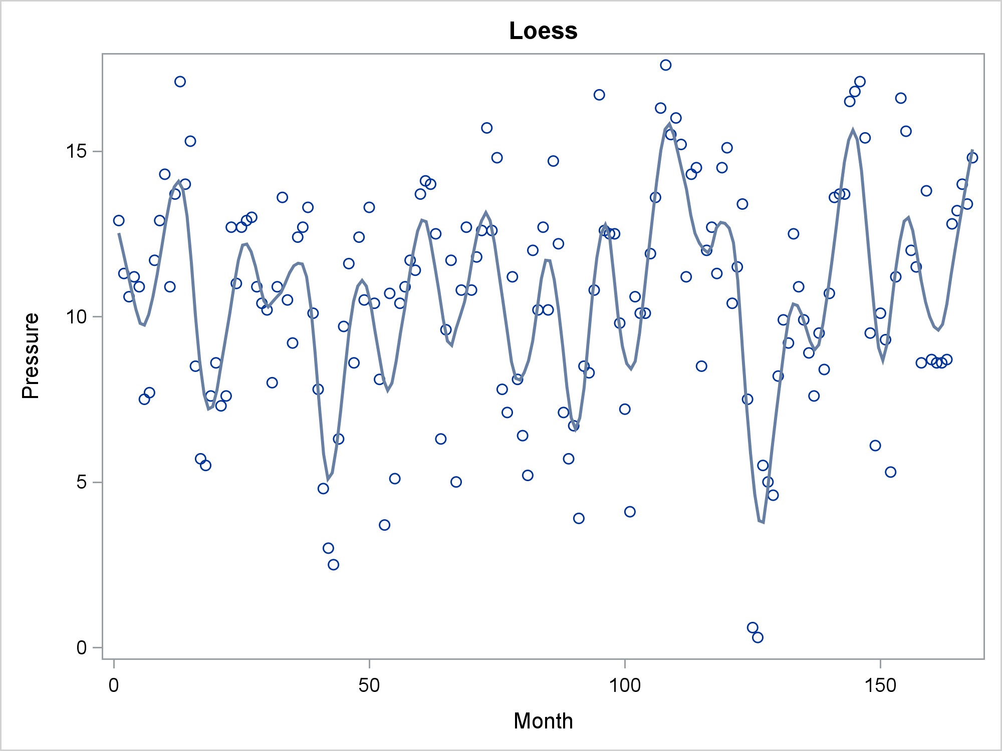
The following step displays a single curve and a scatter plot of points.

proc sgplot data=sashelp.enso noautolegend;
   title 'Loess';
   loess y=Pressure x=Month;
run;

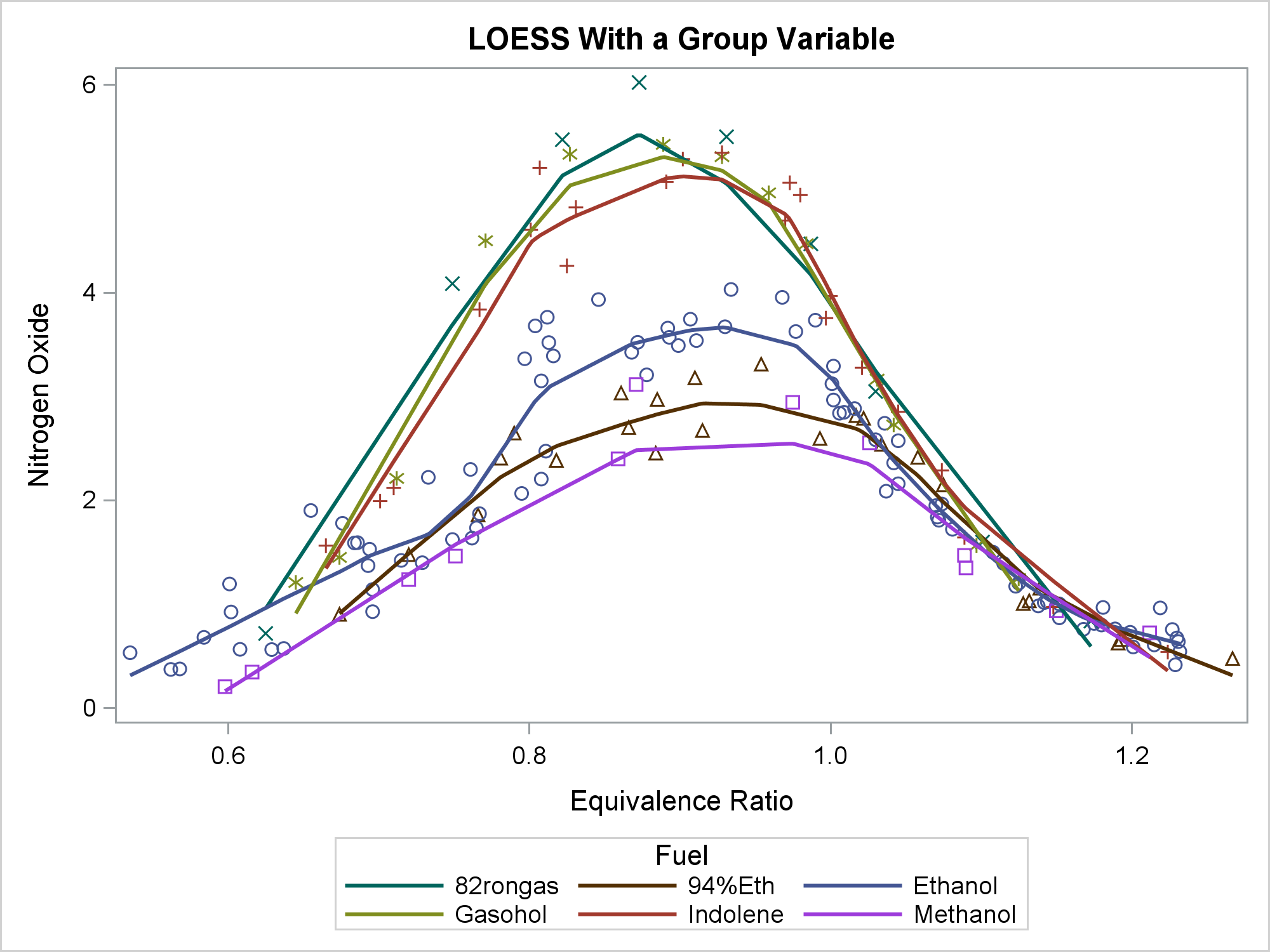
You can specify the GROUP= option in the LOESS statement to get a separate fit function for each group. You can also specify ATTRPRIORITY=NONE in the ODS GRAPHICS statement and a STYLEATTRS statement to vary the markers for each group while using solid lines.

ods graphics on / attrpriority=none;
proc sgplot data=sashelp.gas;
   title 'LOESS With a Group Variable';
   styleattrs datalinepatterns=(solid);
   loess y=nox x=eqratio / group=fuel;
run;

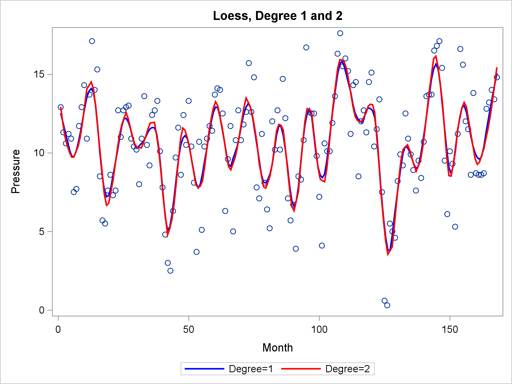
The DEGREE= option specifies the degree of the local polynomials to use for each local regression. Specify either 1 (linear fit, the default) or 2 (quadratic fit). The results are often similar.

proc sgplot data=sashelp.enso;
   title 'Loess, Degree 1 and 2';
   loess y=Pressure x=Month / degree=1 lineattrs=(color=blue) legendlabel='Degree=1';
   loess y=Pressure x=Month / degree=2 lineattrs=(color=red)  legendlabel='Degree=2' nomarkers;
run;

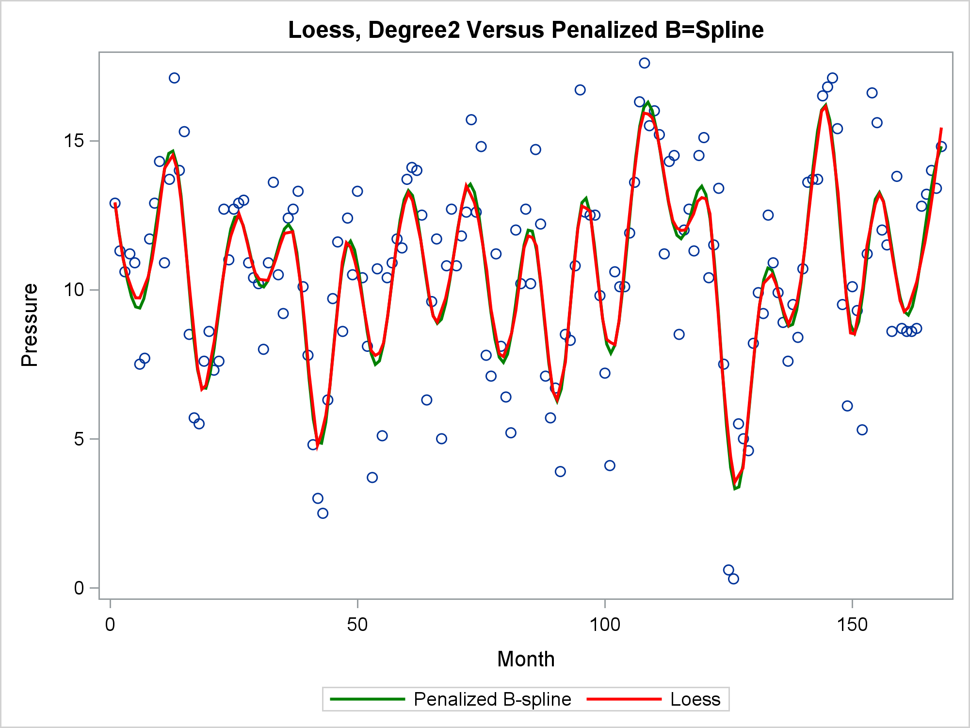
In many cases, the LOESS and PBSPLINE statements produce similar results.

proc sgplot data=sashelp.enso;
   title 'Loess, Degree2 Versus Penalized B=Spline';
   pbspline y=Pressure x=Month /          lineattrs=(color=green);
   loess    y=Pressure x=Month / degree=2 lineattrs=(color=red) nomarkers;
run;

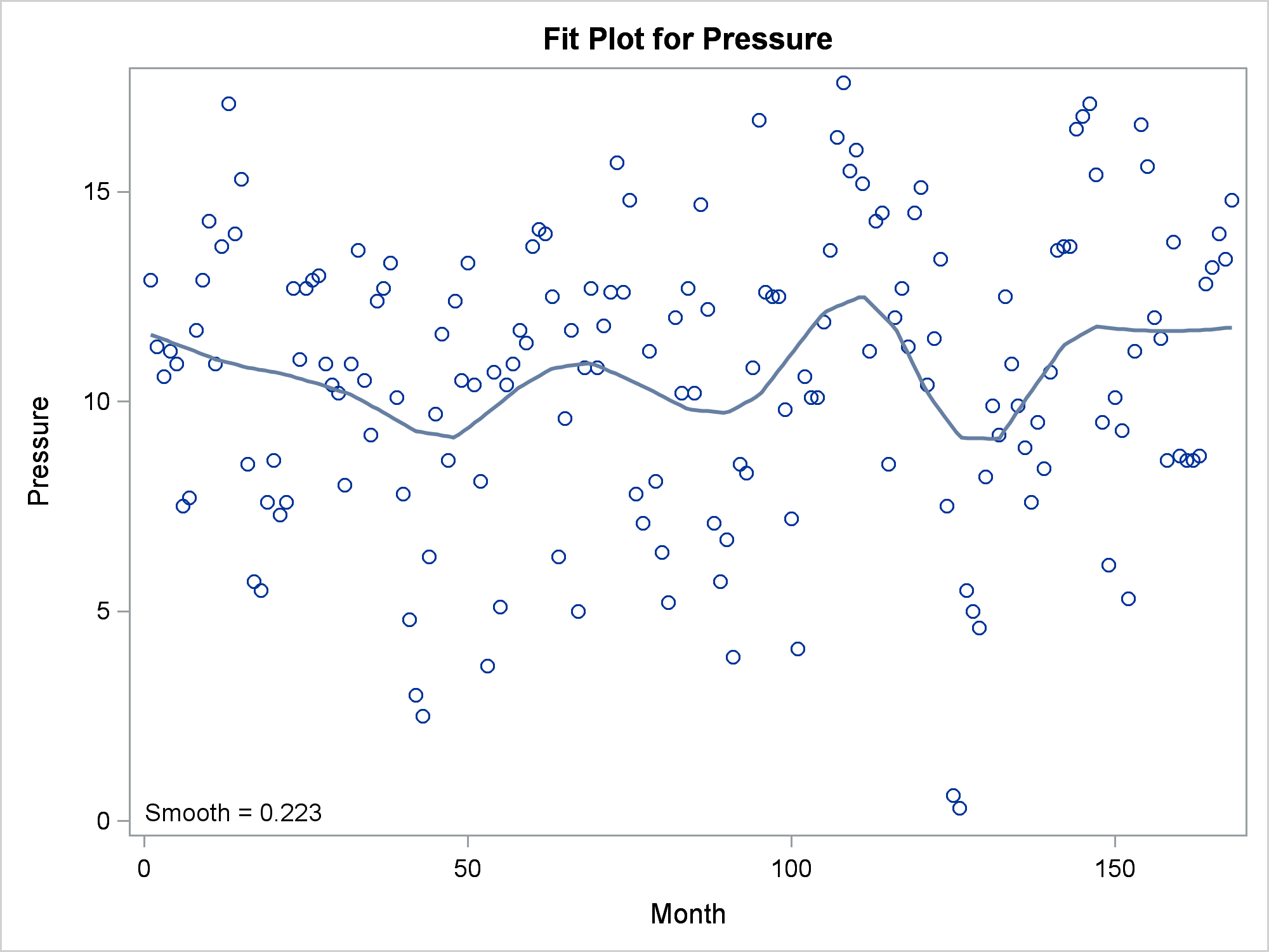
If you want more control over the smoothing options, you can use PROC LOESS. The Sashelp.ENSO data set provides a particularly nice example since the smoothing parameter has both a local and a global optimum. The global optimum shows the effect of seasons, whereas the local optimum shows the effect of El Nino. By default, PROC LOESS finds the local optimum for this data set.

proc loess data=sashelp.enso;
   title 'PROC LOESS, Local Optimum';
   model Pressure = Month;
   ods select fitplot;
run;

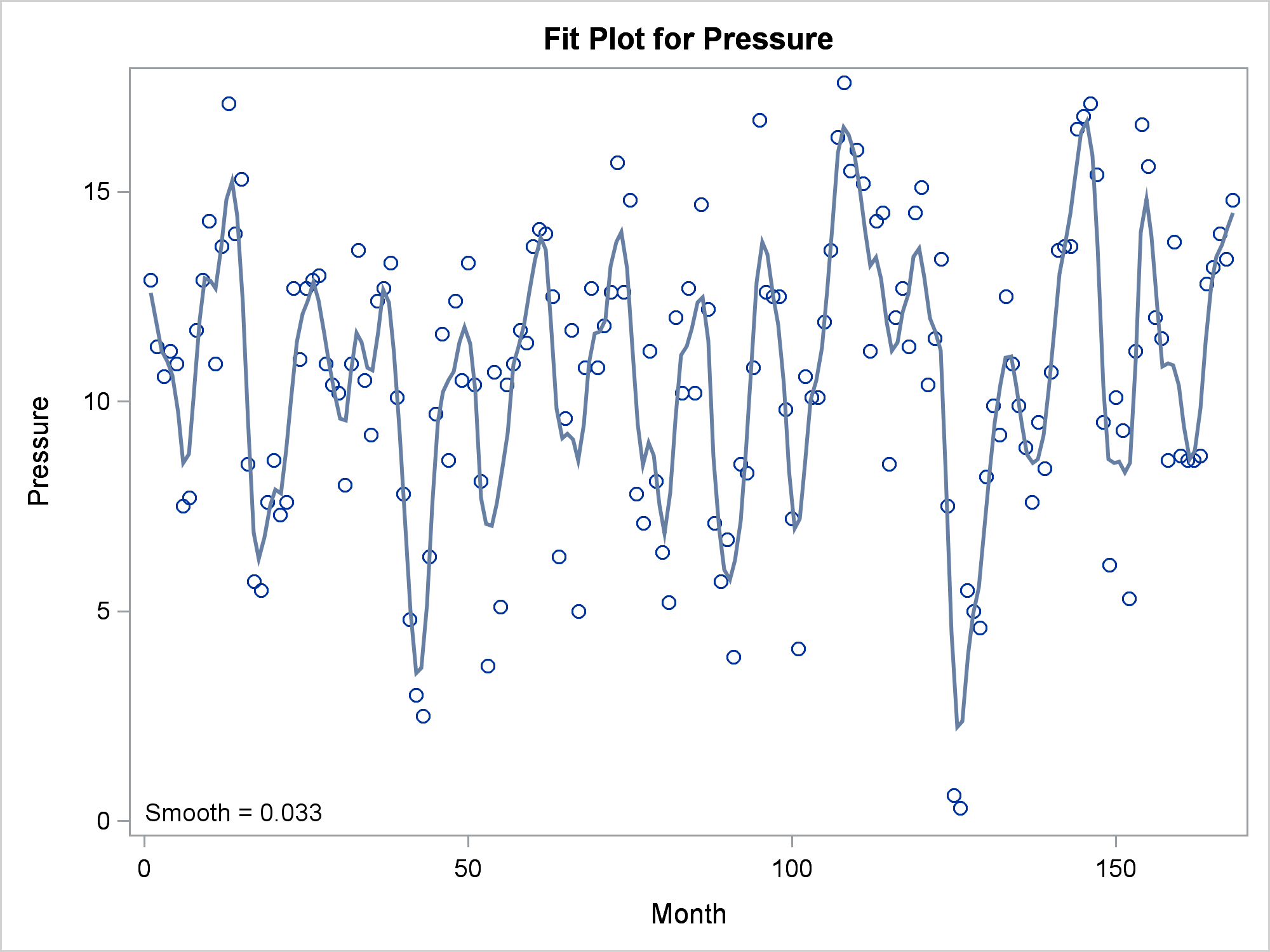
There are many ways you can force it to find the global optimum. This next example specifies a generalized cross-validation criterion and the range for the smoothing parameter.

proc loess data=sashelp.enso;
   title 'PROC LOESS, Global Optimum';
   model Pressure = Month / select=gcv(range(0,0.5));
   ods select fitplot;
run;

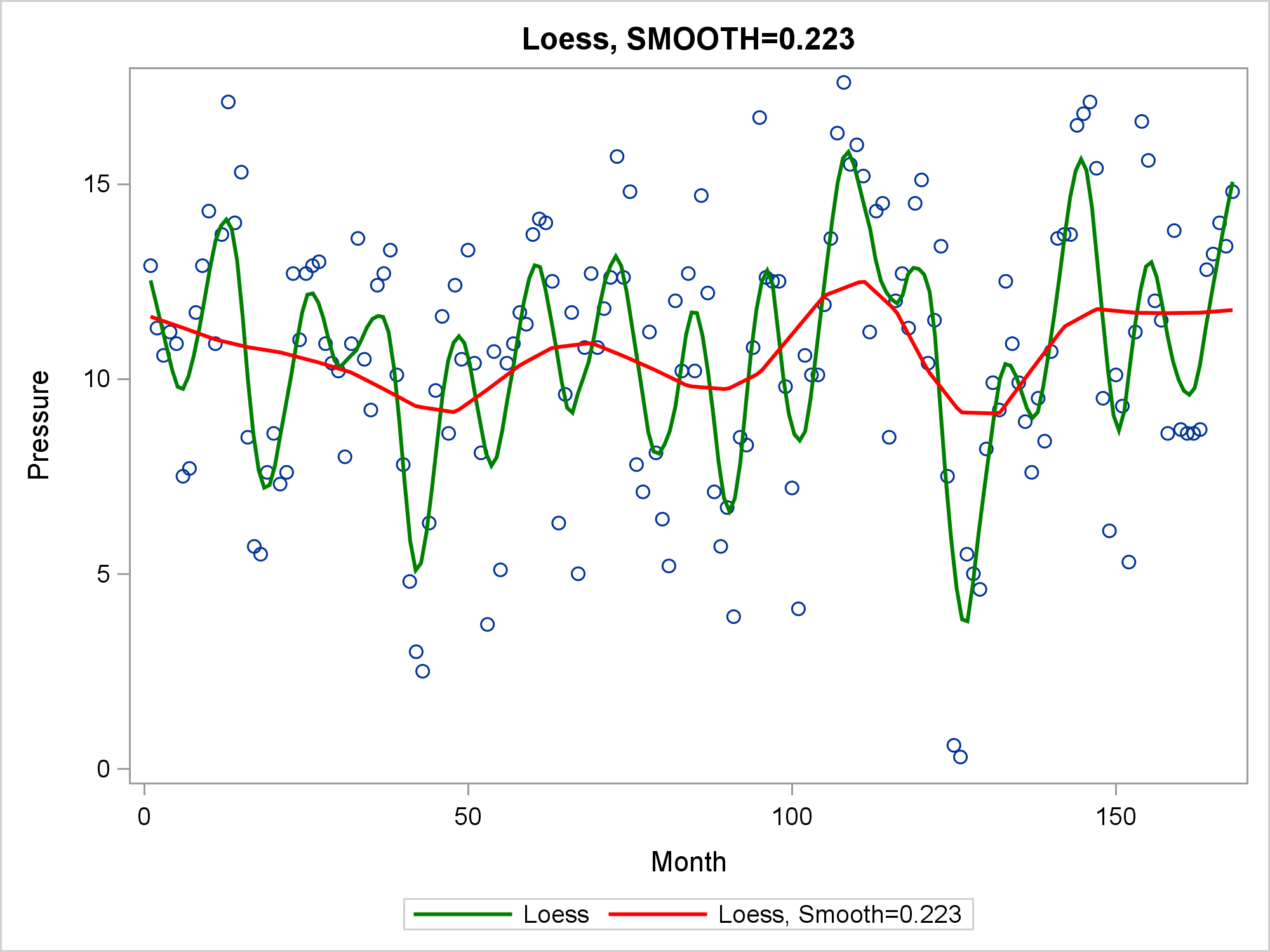
Then you can specify the smoothing parameter in a LOESS statement in PROC SGPLOT. The LOESS statement in PROC SGPLOT uses different default options than PROC LOESS, so this example forces PROC SGPLOT's LOESS statement to find the local optimum, which is displayed along with the global optimum.

proc sgplot data=sashelp.enso;
   title 'Loess, SMOOTH=0.223';
   loess y=Pressure x=Month / degree=1 lineattrs=(color=green);
   loess y=Pressure x=Month / degree=1 lineattrs=(color=red) nomarkers smooth=0.223;
run;

You can additionally specify INTERPOLATION=LINEAR or INTERPOLATION=CUBIC to control the degree of the interpolating polynomials (not shown here).

Linear modeling procedures, such as PROC REG, use loess to find trends in residuals. These trends can help you identify lack of fit and build better models.

proc reg data=sashelp.baseball plots=residuals(smooth);
   ods select residualplot;
   id name team league;
   model logSalary = nhits nruns nrbi nbb yrmajor crhits;
quit;

References

Cleveland,W. S., Devlin, S. J., and Grosse, E. (1988). "Regression by Local Fitting." Journal of Econometrics 37:87-114.

Cleveland, W. S., and Grosse, E. (1991). "Computational Methods for Local Regression." Statistics and Computing 1:47-62.

Cleveland, W. S., Grosse, E., and Shyu, M.-J. (1992). "A Package of C and Fortran Routines for Fitting Local Regression Models." Unpublished manuscript.