Authors: Subbu Pazhani and Rob Pratt

Large-scale real-world optimization problems with advanced business rules are often difficult to solve with standalone traditional optimization algorithms. Metaheuristic algorithms often complement these traditional optimization techniques. These are a class of powerful and flexible algorithms designed to address complex optimization problems, which traditional methods often struggle to solve optimally. They act as a framework for guiding the search process by using problem-specific search methods. These algorithms provide a flexible way to search large solution spaces and quickly identify feasible options. They also refine the most promising ones to find good initial solutions within a reasonable computational time. Traditional optimization techniques further improve and optimize this solution. In this post, we demonstrate a Simulated Annealing (SA) metaheuristic algorithm to solve the Traveling Salesman Problem (TSP) in SAS Optimization.

Researchers have applied the SA metaheuristic algorithm, a popular search method, to solve various combinatorial optimization problems. People use it especially when working with nonlinear functions and large search spaces. The SA algorithm draws inspiration from the physical annealing processes of heating a material to a high temperature. This enables its atoms to rearrange and then slowly cool, achieving a more stable and lower-energy state. SA mimics this concept to optimization problems where a probabilistic approach is used to explore solutions at higher temperatures. The search gradually cools toward a stable and better solution. A key advantage of SA is its ability to escape local optima by accepting an inferior solution by using a probabilistic rule. This enables it to explore the large search spaces to find better solutions.

Pseudocode of the algorithm

This section details the pseudocode of the algorithm along with the details on the variables used in the algorithm, initialization parameters, initialization step, and the steps in the iterations.

• best_obj: best upper bound
• best_iter: iteration identifier corresponding to the best upper bound
• sa_best_obj: best accepted SA solution
• sa_best_iter: iteration identifier corresponding to the best accepted SA solution
• obj_step: objective of that SA iteration

Initialization parameters

• temp: Temperature
• MAX_STEPS: maximum iterations
• fraction_sa: cooling scheme
• max_cons_obj: maximum allowable consecutive solutions where the best_obj of this iteration is the same as the best_obj of the previous iteration

Initialization step

• Generate an initial solution string randomly or by using any heuristic and compute its obj_step.
• Set best_obj, best_iter, sa_best_obj, sa_best_iter based on the initial solution.

Iterations:

done = 0
do until (done = 1)
   /* Generate a new neighbor solution from the string corresponding to sa_best_iter */
   if obj_step < best_obj
      Update best_obj, best_iter, sa_best_obj, sa_best_iter
   else
   /* Compute acceptance probability to accept or reject inferior solution */
   if acceptance probability < rand(0,1)
      /* Accept the inferior neighbor solution */
   /* Compute number of consecutive best_obj solutions (sa_cons_obj_count) */
   if sa_cons_obj_count > max_cons_obj
      sa_best_iter = best_iter
      sa_best_obj = best_obj
   else
      sa_cons_obj_count = 0
 
   /* If stopping criteria met (number of iterations) */
      done = 1
end;

Input data

To illustrate the SA algorithm and its usefulness, we consider an example from the Traveling Salesman Tour of US Capital Cities. This scenario involves traveling the fewest miles to visit all the capital cities in the US states (and the District of Columbia), excluding Alaska and Hawaii.

PROC OPTMODEL code

The model is coded and solved by using the OPTMODEL procedure in SAS Optimization. We begin by defining the index sets and parameters for the TSP problem and by using a READ DATA statement to read data into the index sets and parameters.

proc optmodel;
   /* Declare parameters and read data */
   set <str,str> NODEPAIRS;
   set NODES = union {<i,j> in NODEPAIRS} {i,j};
   num distance{NODEPAIRS};
   num node_id{NODES};
   num id init 1;
   read data CitiesDist (where=(upcase(city1) ne upcase(city2))) 
      into NODEPAIRS=[city1 city2] distance; 
   set  NUM_NODES = 1..CARD(NODES);
   for {n in NODES} do;
      node_id[n] = id;
      id = id + 1;
   end;

The next line calls a macro named sa_tsp_dec, which defines index sets and variables needed for the SA algorithm:

%sa_tsp_dec();

%macro sa_tsp_dec(
);
 
   /* Simulated Annealing - index sets and variables */
   set MAX_STEPS = 1..20000; 
   set NODES_TMP;
   set UPDATE_SET;
   str sa_tsp_tour{MAX_STEPS,NUM_NODES};
   num infinity = constant('BIG');
   num fraction_sa init 0;
   num temp init 1;
   num obj_step{MAX_STEPS};
   num best_obj_step{MAX_STEPS};
   num sa_best_obj_step{MAX_STEPS};
   num best_obj init infinity;
   num best_iter init 1;
   num sa_best_obj init infinity;
   num sa_best_iter init 1;
   num sa_starttime;
   num sa_endtime;
   num sa_runtime init 0;
   num sa_cons_obj_count init 0;
   num max_cons_obj = 10;
   num node1; 
   num node2; 
   str pair1; 
   str pair2; 
   num min_dist;
   num this_node_dist;
   num next_i{i in NUM_NODES} = if i < card(NUM_NODES) then i+1 else 1;
   str next_node;
   num max_node;
   num size_update_set;
   num dec_roundoff = 0.1;
   num inv_mutation_threhold = 0.1;
   num min_temp = 0.01;
   call streaminit(12345678);
 
%mend sa_tsp_dec;

The following set of code executes the first iteration of the SA algorithm. The initial solution string is generated by using the nearest neighborhood method (defined in the sa_nneighbor macro). Then the objective value of this solution string is evaluated by using the sa_compute_obj macro. The system updates this as the best objective and best iteration variables at both the global and SA algorithm levels. Iteration 2 receives this solution string as its best solution.

sa_starttime = time();
   /* Initializing Iteration 1 */
   for {st_sa in {1}} do; 
      /* Generating a initial solution using nearest neighborhood method */
      %sa_nneighbor(); 
 
      /* Evaluating objective function value */
      %sa_compute_obj();
 
      /* Updating best objective and best iteration variables 
         - both at the global level and the SA algorithm level */
      best_obj = obj_step[st_sa];
      best_iter = st_sa;
      sa_best_obj = obj_step[st_sa];
      sa_best_iter = st_sa;
 
      /* Reporting variables */
      best_obj_step[st_sa] = best_obj;
      sa_best_obj_step[st_sa] = sa_best_obj;
 
   end;

%macro sa_nneighbor(
);
 
   NODES_TMP = NODES;
   for {n in NODES: node_id[n] = 1} do;
      sa_tsp_tour[st_sa,node_id[n]] = n;
      NODES_TMP = NODES diff {n};
      leave;
   end;
   id = 1;
   do while (CARD(NODES_TMP)>=1);
      min_dist = infinity;
      for {n1 in NODES_TMP} do;
         this_node_dist = distance[sa_tsp_tour[st_sa,id],n1];
         if min_dist >= this_node_dist then do;
            min_dist = this_node_dist;
            next_node = n1;
         end;
      end;
      id = id + 1;
      sa_tsp_tour[st_sa,id] = next_node;
      NODES_TMP = NODES_TMP diff {next_node};
   end;
 
%mend sa_nneighbor;

%macro sa_compute_obj(
);
 
   obj_step[st_sa] = sum{i in NUM_NODES} distance[sa_tsp_tour[st_sa,i],sa_tsp_tour[st_sa,next_i[i]]];
 
%mend sa_compute_obj;

The next set of statements is a loop for running the SA algorithm iterations. In each iteration, we reduce the annealing (cooling) temperature, generate a neighborhood solution by perturbing the best solution string at the SA algorithm level, evaluate its objective function value, update the best objective and best iteration variables at the global level, and update the best objective and best iteration variables at the SA algorithm level based on the probabilistic acceptance criteria. The algorithm then computes the number of best consecutive solutions, compares it with the maximum allowable consecutive solutions, and resets the best solution string at the SA algorithm level or updates the variable for the number of best consecutive solutions.

for {st_sa in MAX_STEPS: st_sa > 1} do;
 
      /* Computing the cooling temperature step */
      fraction_sa = st_sa / CARD(MAX_STEPS); 
 
      /* Computing temperature */
      temp = max(min_temp,1 - fraction_sa);
 
      /* Generating a neighborhood solution */
      if temp >= inv_mutation_threhold then do; 
         %sa_inverse();
      end;
      else do; 
         %sa_swap(); 
      end;
 
      /* Evaluating objective function value */
      %sa_compute_obj();
 
      /* Updating best objective and best iteration variables 
         - both at the global level and the SA algorithm level */
      if (obj_step[st_sa] < best_obj) then do; best_obj = obj_step[st_sa]; best_iter = st_sa; sa_best_obj = obj_step[st_sa]; sa_best_iter = st_sa; end; else if (obj_step[st_sa] > best_obj and 
         exp(-((obj_step[st_sa]-best_obj) / obj_step[st_sa]) / temp ) > rand("Uniform")) then do; 
         sa_best_obj = obj_step[st_sa];
         sa_best_iter = st_sa;
      end;
      else do;
         best_obj = best_obj;
         best_iter = best_iter;
         sa_best_obj = sa_best_obj;
         sa_best_iter = sa_best_iter;
      end; 
 
      /* Computing number of consecutive same best solution */
      if (round(obj_step[st_sa-1],dec_roundoff) 
        = round(obj_step[st_sa],dec_roundoff) or obj_step[st_sa] > best_obj) then do;
         sa_cons_obj_count = sa_cons_obj_count + 1;
      end;
      else sa_cons_obj_count = 0; 
      if sa_cons_obj_count > max_cons_obj then do;
         sa_best_iter = best_iter;
         sa_best_obj = best_obj;
      end;
 
      /* Reporting variables */
      best_obj_step[st_sa] = best_obj;
      sa_best_obj_step[st_sa] = sa_best_obj;
 
   end;

The following two macros (sa_inverse and sa_swap) illustrate the inverse mutation scheme and the swap mutation scheme for generating a neighborhood solution.

%macro sa_inverse(
);
   /* Entering inverse mutation */
   do until (node1 ne node2);
      node1 = rand("integer",1,CARD(NUM_NODES)); 
      node2 = rand("integer",1,CARD(NUM_NODES)); 
   end;
 
   /* Initializing the string to SA best iteration */
   for {i in NUM_NODES} sa_tsp_tour[st_sa,i] = sa_tsp_tour[sa_best_iter,i];
 
   /* Performing inverse mutation */
   max_node = max(node1,node2); 
   UPDATE_SET = if node1 < node2 then node1..node2 else node2..node1;
   size_update_set = CARD(UPDATE_SET);
   id = 1; 
   do while (id <= size_update_set);
      for {i in UPDATE_SET} do;
         sa_tsp_tour[st_sa,i] = sa_tsp_tour[sa_best_iter,max_node-id+1];
         id = id + 1;
      end;
   end;
 
%mend sa_inverse;

%macro sa_swap(
);
 
   /* Entering pairwise mutation */
   do until (node1 ne node2);
      node1 = rand("integer",1,CARD(NUM_NODES)); 
      node2 = rand("integer",1,CARD(NUM_NODES)); 
   end;
 
   pair1 = sa_tsp_tour[sa_best_iter,node2]; 
   pair2 = sa_tsp_tour[sa_best_iter,node1]; 
 
   for {i in NUM_NODES} do;
      if i = node1 then sa_tsp_tour[st_sa,i] = pair1;
      else if i = node2 then sa_tsp_tour[st_sa,i] = pair2;
      else sa_tsp_tour[st_sa,i] = sa_tsp_tour[sa_best_iter,i];
   end;
 
%mend sa_swap;

The following statement is used to extract the best solution from the SA algorithm and output the resulting solution:

 /* Run time of the SA algorithm */
   sa_endtime = time();
   sa_runtime = intck('second',sa_starttime,sa_endtime);
   put sa_runtime=;
 
   /* Creating output table */
   set <str,str> TSPEDGES;
   TSPEDGES = union{i in NUM_NODES} {<sa_tsp_tour[sa_best_iter,i],sa_tsp_tour[sa_best_iter,next_i[i]]>};
   create data TSPTourLinks from [city1 city2] = TSPEDGES distance;
   create data TSPSAIterations from [Iteration_no] = MAX_STEPS best_obj_step sa_best_obj_step;
 
quit;

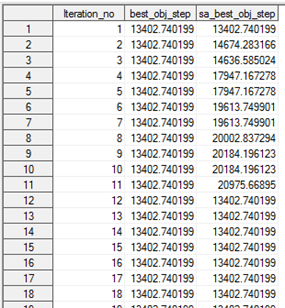
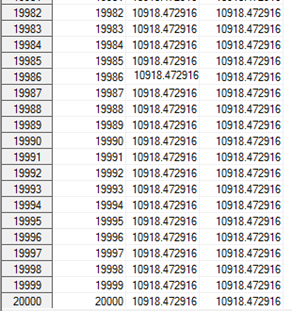
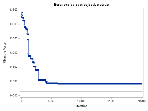
We execute the SA algorithm, coded within PROC OPTMODEL, by using the input data. The optimal objective value of the problem is 10,635.09 and can be found in the Traveling Salesman Tour of US Capital Cities. The SA algorithm started with a solution that had an objective function value of 13,402.74. It terminated with a solution with an objective function value of 10,918.47 (a gap of 2.66% from the optimal objective value). The algorithm took 4 seconds to run the set of 20000 iterations. Table 1 shows a few iterations with starting solutions. While Table 2 shows a few iterations with the final solution from the Tspsaiterations table.

The choice of neighborhood mutation schemes directly influences the quality of solutions the SA algorithm generates. These include inverse and swap mutations, as well as the selection of runtime parameters, including the number of iterations, cooling scheme, and mutation threshold. Fine-tuning these aspects can lead to a more robust search process, improving both solution diversity and overall effectiveness in tackling complex optimization problems. However, fine-tuning these aspects is problem-specific and requires conducting experiments to determine appropriate settings.

Plots of solutions

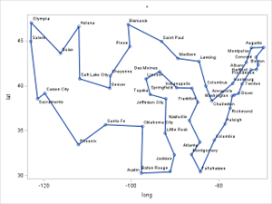
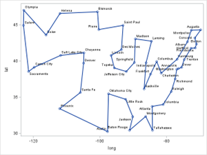
The statements to produce a graphical display of the solution can be referred to from the example in the Traveling Salesman Tour of US Capital Cities. Figures 1 and 2 illustrate the optimal solution and the best tour of the capital cities generated by the SA algorithm. As we observe, there are route differences between the optimal solution and the best solution from the SA algorithm.

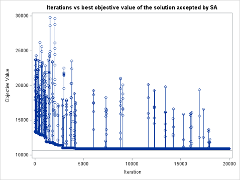
The following two statements plot the iterations. Figure 3 illustrates the progress of the best objective value and the corresponding best objective value for the solution accepted by the SA algorithm (see Figure 4). The iterations versus best objective value corresponding to the solution accepted at the SA algorithm level (refer to Figure 4) show the probabilistic behavior of the algorithm in accepting an inferior solution, showing occasional increases in objective value when inferior solutions are accepted, before resuming improvement. The overall downward trend captures the algorithm’s effectiveness in navigating the solution landscape towards near-optimality.

/* Progress of best objective */
title 'Iterations vs best objective value';
%let optimal = 10635;
proc sgplot data = TSPSAIterations noautolegend;
   step x = Iteration_no y = best_obj_step / markers;
   refline &optimal.;
   xaxis label = 'Iteration';
   yaxis label = 'Objective Value' min = 10500;
run;
 
/* Progress of sa best objective */
title 'Iterations vs best objective value of the solution accepted by SA';
proc sgplot data = TSPSAIterations noautolegend;
   step x = Iteration_no y = sa_best_obj_step / markers;
   refline &optimal.;
   xaxis label = 'Iteration';
   yaxis label = 'Objective Value' min = 10500;
run;

Conclusion

This example illustrates solving a TSP by using an SA algorithm coded and then executed in PROC OPTMODEL. Note that the SA algorithm provides only an approximate solution to the global optimum. However, it could be useful for obtaining a good, feasible solution for a wide variety of complex, real-world problems. Other applications of SA include vehicle routing problems and extensions, supply chain network design, and scheduling problems.

Another extension uses this SA framework in conjunction with state-of-the-art solvers in SAS Optimization. For example, SA fixes some of the complicated variables. Then it solves the optimization model to determine the remaining unfixed variables.

SAS Optimization has specialized solvers for various graph theory, combinatorial optimization, and network analysis algorithms, including TSP.